Empirical Example from Grabowski (2024) Walkthrough

This example presents the basic and advanced options of Blouch and the code below is the complete analysis of the empirical example from Grabowski (in press) on antler size and breeding group evolution.

rm(list=ls())
library(blouch)

Background

Tsuboi et al. (2024) collected an expansive dataset on antler size and body size and generated a new Cervidae phylogeny to test the hypothesis of Gould (1973) that the elaborate antlers of the Irish Elk were the result of a positive allometric relationship with body size. I supplemented this dataset with data on Cervidae breeding group size categories from Plard et al. (2011) and Clutton-Brock et al. (1980) to test the hypothesis that antler size is influenced by sexual selection by using breeding group size as a predictor of antler size.

As formulated by Clutton-Brock et al. (1980), the specific hypothesis is that the relatively larger antlers of larger bodied deer are the result of more intense sexual selection that comes along with their tendency to live in larger breeding groups. Following Tsuboi et al. (2024) the relationship between posterior skull length and antler volume is hypothesized to be allometric and thus the direct effect model is a reasonable choice. Following Hansen (2014), as sexual selection would likely not cause an immediate change in either body size or antler volume, the multi-optima model is indicated.

The hypothesized causal relationship between these three variables is shown in the directed acyclic graph (DAG) below.

set.seed(11)
ggplot2::theme_set(ggdag::theme_dag())

dag<-ggdag::ggdag(ggdag::dagify(
  A ~ B,
  P ~ B,
  A ~ P,
  A ~ u,
  B ~ u,
  P ~ u,
  u ~ R
  ))

dag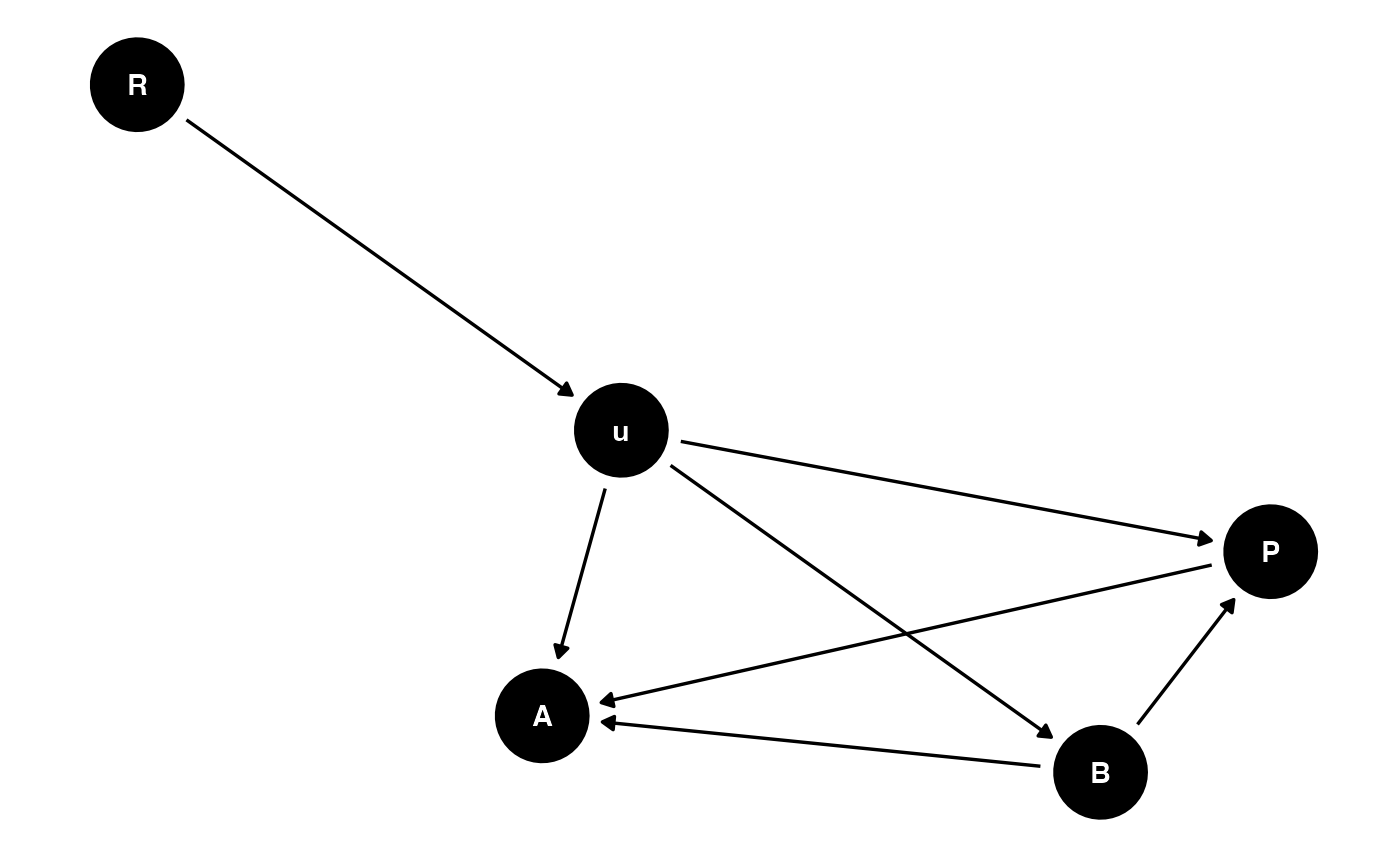

Blouch uses RStan to implement Stan. The following code enables some compiler optimizations to improve the estimation speed of the model, and is taken from: https://github.com/stan-dev/rstan/wiki/RStan-Getting-Started.

#options(mc.cores = parallel::detectCores())
options(mc.cores = 2) #2 For R package checks - use line above on your own machine
rstan::rstan_options(auto_write = TRUE)

dotR <- file.path(Sys.getenv("HOME"), ".R")
if (!file.exists(dotR)) dir.create(dotR)
M <- file.path(dotR, "Makevars")
if (!file.exists(M)) file.create(M)
arch <- ifelse(R.version$arch == "aarch64", "arm64", "x86_64")
cat(paste("\nCXX14FLAGS += -O3 -mtune=native -arch", arch, "-ftemplate-depth-256"),
    file = M, sep = "\n", append = FALSE)

Load datasets

First, load the tree from Tsuboi et al. (2024) and the dataset. Original ata from Tsuboi et al. (2024) is available at DRYAD: https://doi.org/10.5061/dryad.kh18932dt, and dataset including breeding group regims is included in the Blouch package.

########################################################################################################
set.seed(10)

########################################################################################################
#For execution on a local, multicore CPU with excess RAM we recommend calling
options(mc.cores = parallel::detectCores())
rstan::rstan_options(auto_write = TRUE)

########################################################################################################

#Remove Muntiacus_atherodes, Elaphodus_cephalophus - rudamentary and female Rangifer - following Tsuboi et al. (2024)
antler.data<-dplyr::filter(antler.data,Genus_Species != "Sinomegaloceros_yabei" & ! Genus_Species =="Alces_alces_gigas"  & ! Genus_Species == "Muntiacus_truongsonensis" & ! Genus_Species ==  "Mazama_temama"& ! Genus_Species ==  "Muntiacus_feae" & ! Genus_Species ==  "Muntiacus_atherodes" & ! Genus_Species ==  "Elaphodus_cephalophus")

Combine data and tree and paint regimes on tree.

Next we will use the treeplyr package (Uyeda and Harmon, 2014) make.treedata function to combine the data and tree based on the taxa names. See https://github.com/uyedaj/treeplyr for more on this package.

cervid.trdata <- treeplyr::make.treedata(cervidae.tree, antler.data,name_column="Genus_Species")

cervid.trdata<-dplyr::filter(cervid.trdata,!(is.na(log_ant_vol)) & !(is.na(log_psl)))
#cervid.trdata<-dplyr::mutate(cervid.trdata,mc.log_psl=cervid.trdata$dat$log_psl-(mean(cervid.trdata$dat$log_psl)))

cervid.trdata<-dplyr::mutate(cervid.trdata,me.log_ant_vol=cervid.trdata$dat$log_vol_var_est/cervid.trdata$dat$n)
cervid.trdata<-dplyr::mutate(cervid.trdata,me.log_psl=cervid.trdata$dat$log_psl_var_est/cervid.trdata$dat$n)
cervid.trdata<-dplyr::filter(cervid.trdata,!(is.na(me.log_ant_vol)) & !(is.na(me.log_psl)))

#Mean standardize predictor
cervid.trdata$dat$mc_log_psl<-cervid.trdata$dat$log_psl-mean(cervid.trdata$dat$log_psl)
cervid.trdata$dat$mc_log_ant_vol<-cervid.trdata$dat$log_ant_vol-mean(cervid.trdata$dat$log_ant_vol)


########################################################################################################
#Main text analysis adding in BGS effect as adaptive predictor
########################################################################################################
cervid.trdata.BGS<-dplyr::filter(cervid.trdata,!(is.na(BGS)))

#Rescale tree height to 1
l.tree<-max(ape::branching.times(cervid.trdata.BGS$phy))
cervid.trdata.BGS$phy$edge.length<-cervid.trdata.BGS$phy$edge.length/l.tree ## rescale tree to height 1
max(ape::branching.times(cervid.trdata.BGS$phy))
#> [1] 1

tip.label<-cervid.trdata.BGS$phy$tip.label
phy<-cervid.trdata.BGS$phy
#Dmat<-cophenetic(phy) #Time separating tips, same as tij matrix in Slouch/Blouch code

Next we will reconstruct the breeding group size regimes on the phylogeny using the ace function from the R package ape. Then we will calculate the most likely regime at each node using maximum likelihood estimation (Pagel 1994) and add these to the internal nodes of our phylogeny. We will use the equal-rates model (ER), the all-rates different model (ARD), and the symmetrical model (SYM), and then compare them using AICc.

########################################################################################################
#Regime reconstruction using ace from ape
reconstructed.BGS.ER <- ape::ace(as.factor(cervid.trdata.BGS$dat$BGS), cervid.trdata.BGS$phy, type = "d", model="ER")
reconstructed.BGS.ARD <- ape::ace(as.factor(cervid.trdata.BGS$dat$BGS), cervid.trdata.BGS$phy, type = "d", model="ARD")
reconstructed.BGS.SYM <- ape::ace(as.factor(cervid.trdata.BGS$dat$BGS), cervid.trdata.BGS$phy, type = "d", model="SYM")

AIC(reconstructed.BGS.ER)
#> [1] 61.86089
AIC(reconstructed.BGS.ARD)
#> [1] 71.36351
AIC(reconstructed.BGS.SYM)
#> [1] 65.36549

#The lowest AIC is for the equal rates model so we will use that in our analysis
reconstructed.BGS<-reconstructed.BGS.ER

internal.regimes.BGS<- apply(reconstructed.BGS$lik.anc, 
                                     1, 
                                     function(e) colnames(reconstructed.BGS$lik.anc)[which.max(e)])

#Assign internal regimes to node.label on phylogeny - for use by Blouch prep functions
cervid.trdata.BGS$phy$node.label<-as.factor(internal.regimes.BGS)

Now lets check if these regime placements make sense

########################################################################################################
#Check if manual setting code worked - not needed for setting regimes
shifts.total<-unlist(list(as.factor(cervid.trdata.BGS$dat$BGS),factor(internal.regimes.BGS)))
edge.regimes <- factor(shifts.total[cervid.trdata.BGS$phy$edge[,2]])
print(edge.regimes)
#> 32 33    34 35 36 37 38    39 40                41    42          43       44 
#>  B  B  B  B  B  B  B  B  B  B  B  C  B  A  B  A  B  A  B  B  B  C  B  B  B  C 
#> 45 46 47    48          49 50 51 52 53    54          55       56          57 
#>  C  C  C  C  C  A  C  C  C  C  C  C  C  C  C  C  B  C  C  C  B  C  C  C  C  A 
#>    58 59          
#>  A  A  A  A  A  A 
#> Levels: A B C

reg.colors<-ggsci::pal_aaas("default", alpha = 1)(length(unique(edge.regimes)))

plot(cervid.trdata.BGS$phy,edge.color = reg.colors[edge.regimes], edge.width = 1, cex = 0.5)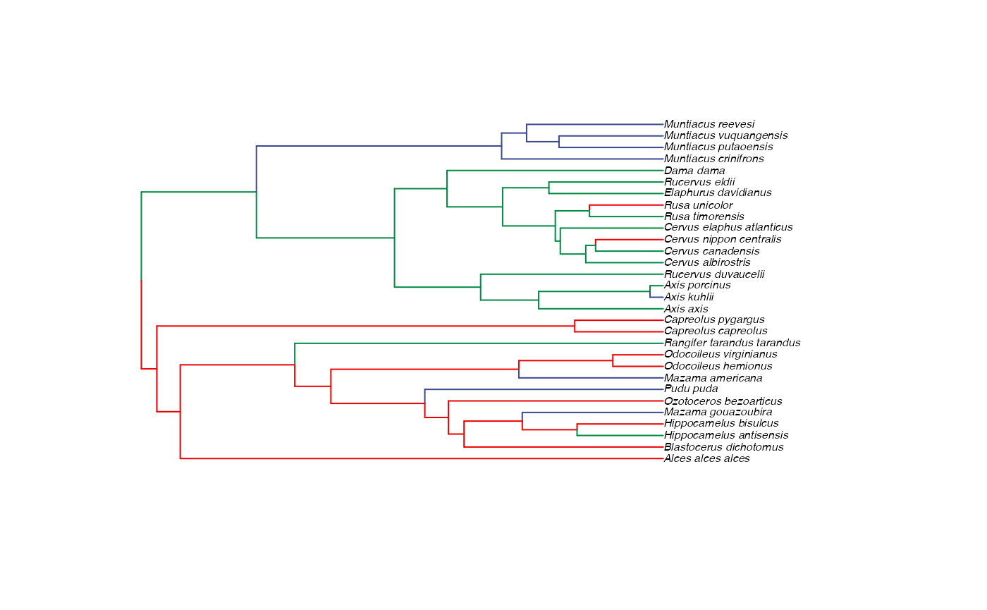

Setup dataset and add measurement errors

Now lets set up the variables - including measurement errors. We could call the data whatever we wanted (e.g “Y_with_error” below), as long as we combine all the data together into one

########################################################################################################
#Setup Measurement Errors - for use with blouchOU_reg_direct
N<-length(cervid.trdata.BGS$phy$tip.label)
Z_direct<-1
Z_X_error<-1
Y_with_error<-cervid.trdata.BGS$dat$mc_log_ant_vol
X_with_error<-cervid.trdata.BGS$dat$mc_log_psl
Y_error<-sqrt(cervid.trdata.BGS$dat$me.log_ant_vol) #Standard error not variance
X_error<-sqrt(cervid.trdata.BGS$dat$me.log_psl) #Standard error not variance
trdata<-cervid.trdata.BGS
regimes_tip <- cervid.trdata.BGS$dat$BGS

Lets add the data to our trdata variable, which already contains the tree

############################################################################################################
#Add errors to trdata file
trdata$dat<-cbind(trdata$dat,data.frame(cbind(Y_with_error,Y_error,X_with_error,X_error)))

Setting Priors

Let’s make a simple plot of data, and look at a simple ordinary least squares regression of Y on X. The intercept and slope values will give us an idea of how to center our priors below.

df<-data.frame(Y=Y_with_error,X=X_with_error)
ols.coef<-summary(lm(Y~X,df))
ols.coef$coefficients[c(1,2)] #Intercept and slope
#> [1] 0.0444186 6.3044512

ols.plot<-ggplot2::ggplot(data=df,ggplot2::aes(x=X,y=Y))+
  ggplot2::geom_point()+
  ggplot2::geom_abline(intercept=ols.coef$coefficients[1],slope=ols.coef$coefficients[2],alpha=0.1)+
  ggplot2::theme_bw()+
  ggplot2::theme(
    panel.grid.major = ggplot2::element_blank(),
    panel.grid.minor = ggplot2::element_blank())

ols.plot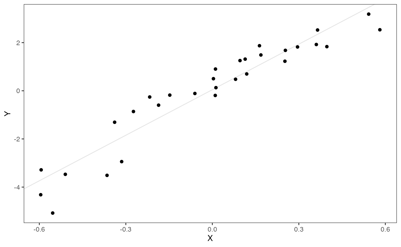

Below are the priors used for this first analysis. See Grabowski (in press) for more on setting these priors, but here our optima (intercept) and slope are informed by the linar model.

############################################################################################################
#Set Priors
hl.prior<-c(log(0.25),0.25)
vy.prior<-10
optima.prior<-c(0.05,0.75) #Informed by linear model above
beta.prior<-c(6.304451,1.75) #Informed by linear model above

Exploring Priors

Lets simulate from our priors to check if these are reasonable values for the intercept and slope - futher below is code for looking at the priors for the other parameters in the model, in the prior vs. posterior plots section. These are the “.sims” values - the priors are based on the intercept and slope of the OLS regression above, with standard deviations set by visualizing the priors versus the data.

Half-life Prior plot

hl.sims<-data.frame(rlnorm(n=1000,meanlog=hl.prior[1],sdlog=hl.prior[2]))
names(hl.sims)<-"prior.hl.sims"

hl.prior.plot<-ggplot2::ggplot()+
  ggplot2::geom_density(ggplot2::aes(prior.hl.sims,fill="prior.hl.sims"),alpha=0.2,data=hl.sims)+
  ggplot2::theme_bw()+
  ggplot2::theme(
    panel.grid.major = ggplot2::element_blank(),
    panel.grid.minor = ggplot2::element_blank())+
  
  #labs(title="Prior vs. Posterior Distribution ",x="Half-life", y = "Density")+
  ggplot2::labs(title="",x="Half-life", y = "Density")+
  
  #scale_fill_manual(labels=c("Posterior","Prior"))+
  ggsci::scale_fill_npg(name="",labels=c("Prior"))

hl.prior.plot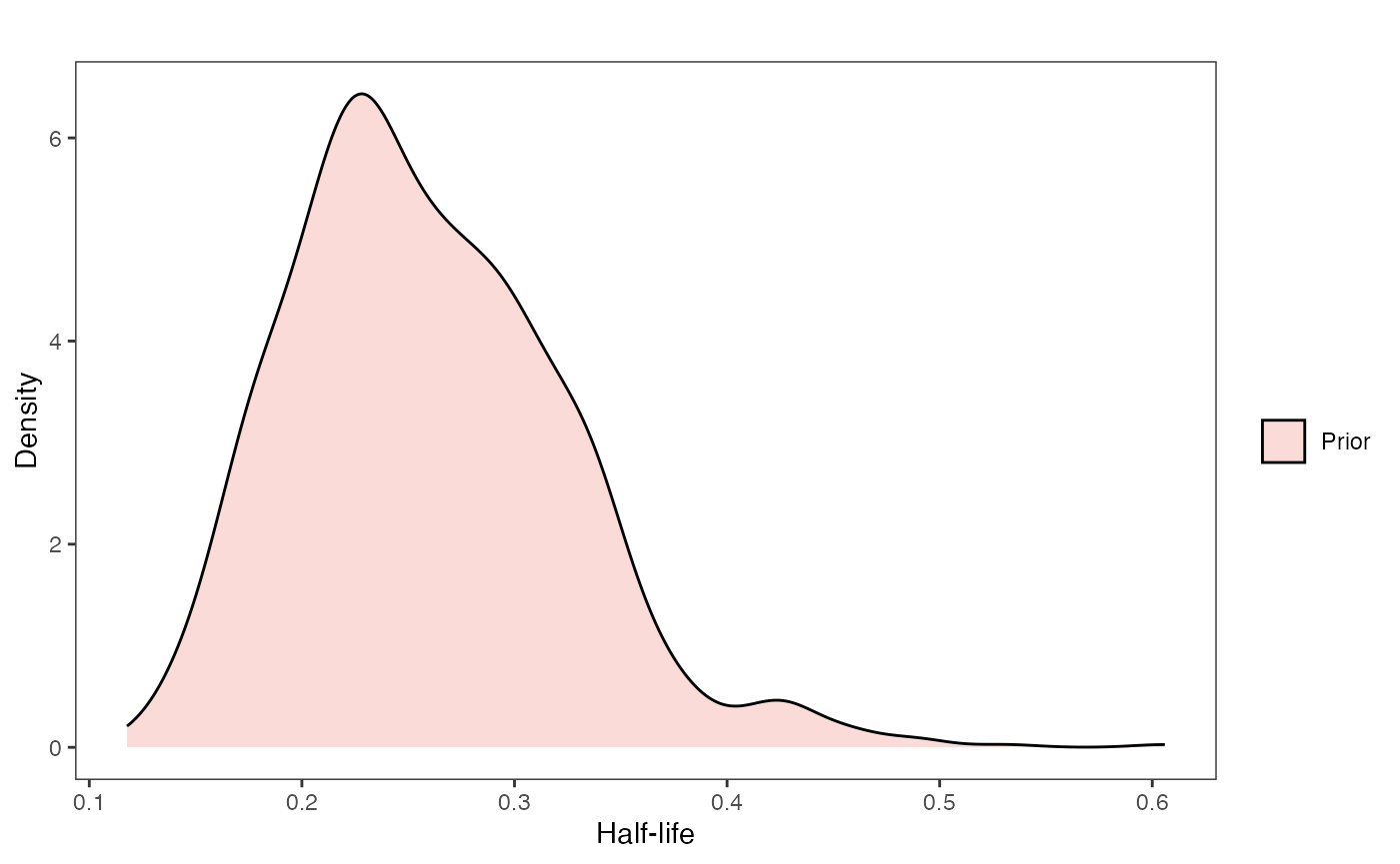

Vy Prior Plot

vy.sims<-rexp(n=1000,rate=vy.prior)
vy.sims<-data.frame(vy.sims)
names(vy.sims)<-"prior.vy.sims"

vy.prior.plot<-ggplot2::ggplot()+
  ggplot2::geom_density(ggplot2::aes(prior.vy.sims,fill="prior.vy.sims"),alpha=0.2,data=vy.sims)+
  ggplot2::theme_bw()+
  ggplot2::theme(
    panel.grid.major = ggplot2::element_blank(),
    panel.grid.minor = ggplot2::element_blank())+
  
  #labs(title="Prior vs. Posterior Distribution ",x="vy", y = "Density")+
  ggplot2::labs(title="",x="vy", y = "Density")+

  #scale_fill_manual(labels=c("Posterior","Prior"))+
  ggsci::scale_fill_npg(name="",labels=c("Prior"))


vy.prior.plot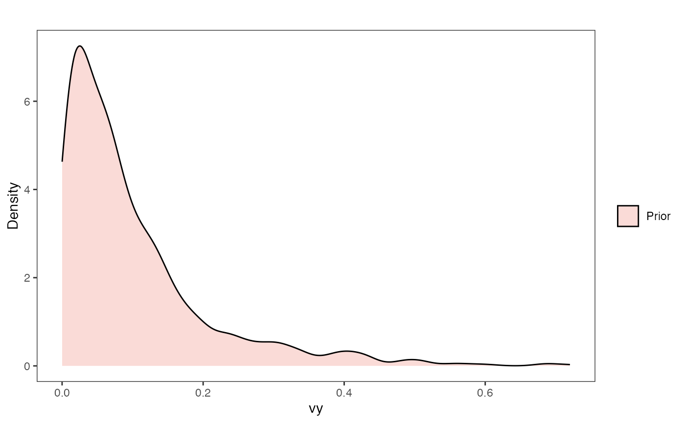

Prior on how shared branch lengths correspond to covariance

hl.sims<-data.frame(rlnorm(n=1000,meanlog=hl.prior[1],sdlog=hl.prior[2]))
vy.sims<-rexp(n=1000,rate=vy.prior)
a.sims<-log(2)/hl.sims
sigma2_y.sims<-vy.sims*(2*(log(2)/hl.sims))
mypal <- ggsci::pal_npg("nrc", alpha = 0.4)(2)

x<-seq(0,1,by=0.01)
df<-data.frame(x)

p<-ggplot2::ggplot(df,ggplot2::aes(x))
for(i in 1:30){
  p<-p+ggplot2::stat_function(fun=function(x,i) {sigma2_y.sims[i,] /(2 * a.sims[i,]) * ((1 - exp(-2 * a.sims[i,] * (1-(x/2)))) * exp(-a.sims[i,] * x))},
                              args=list(i=i),alpha=0.2,lwd=2)}
p<-p+ggplot2::theme_bw()+
  ggplot2::theme(
    panel.grid.major = ggplot2::element_blank(),
    panel.grid.minor = ggplot2::element_blank())+
  ggplot2::labs(title="",x="Time Since MRCA", y = "Covariance")
p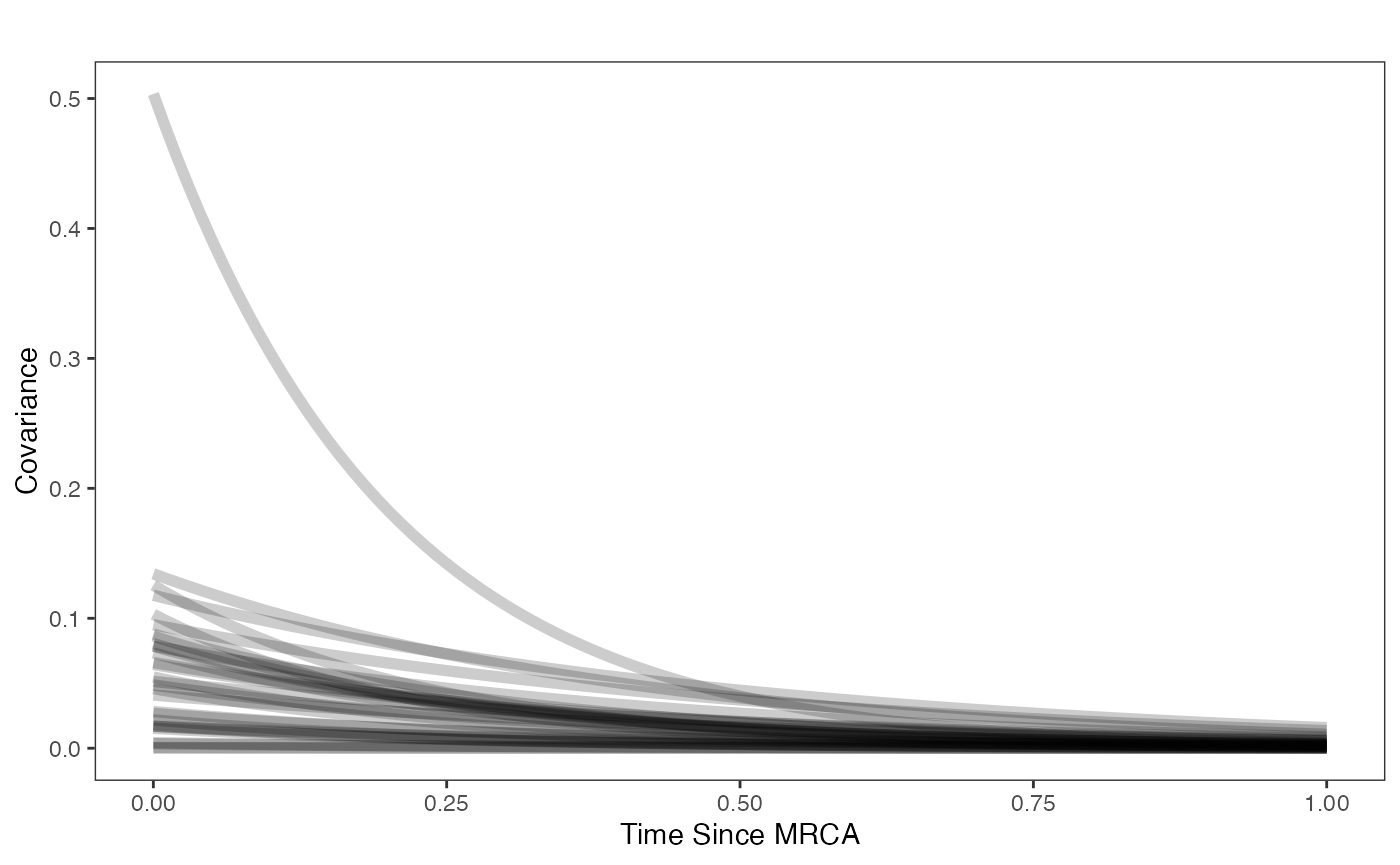

Slope and intercept Prior Plot

optima.sims<-rnorm(100,optima.prior[1],optima.prior[2])
beta.sims<-rnorm(n=100,beta.prior[1],beta.prior[2])

df<-data.frame(Y=trdata$dat$Y_with_error,X=trdata$dat$X_with_error)

slope.plot.1<-ggplot2::ggplot()+
  ggplot2::geom_point(data=df,ggplot2::aes(y=Y,x=X))+
  ggplot2::geom_abline(intercept=optima.sims,slope=beta.sims,alpha=0.15)+ #Prior
  ggplot2::theme_bw()+
  ggplot2::theme(
    panel.grid.major = ggplot2::element_blank(),
    panel.grid.minor = ggplot2::element_blank())+
  ggplot2::ylab("Y") + ggplot2::xlab("X - Direct Effect Model")+
  ggsci::scale_color_npg()

slope.plot.1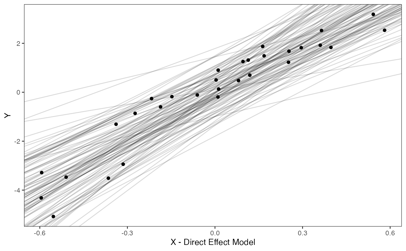

Explore Priors - built in functions

Blouch also contains built in functions to plot the priors, as seen below.

hl.prior.plot.code(hl.prior)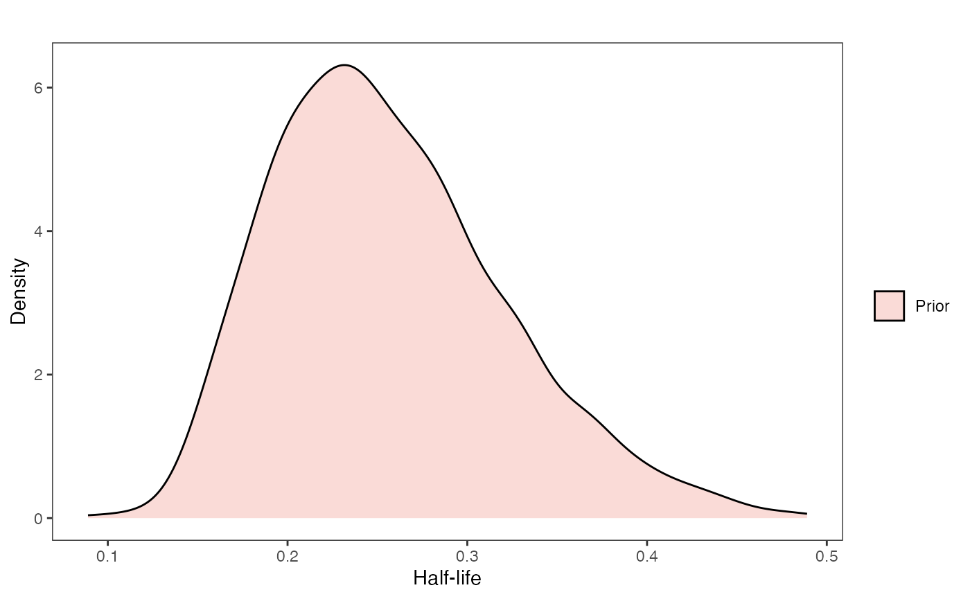

vy.prior.plot.code(vy.prior)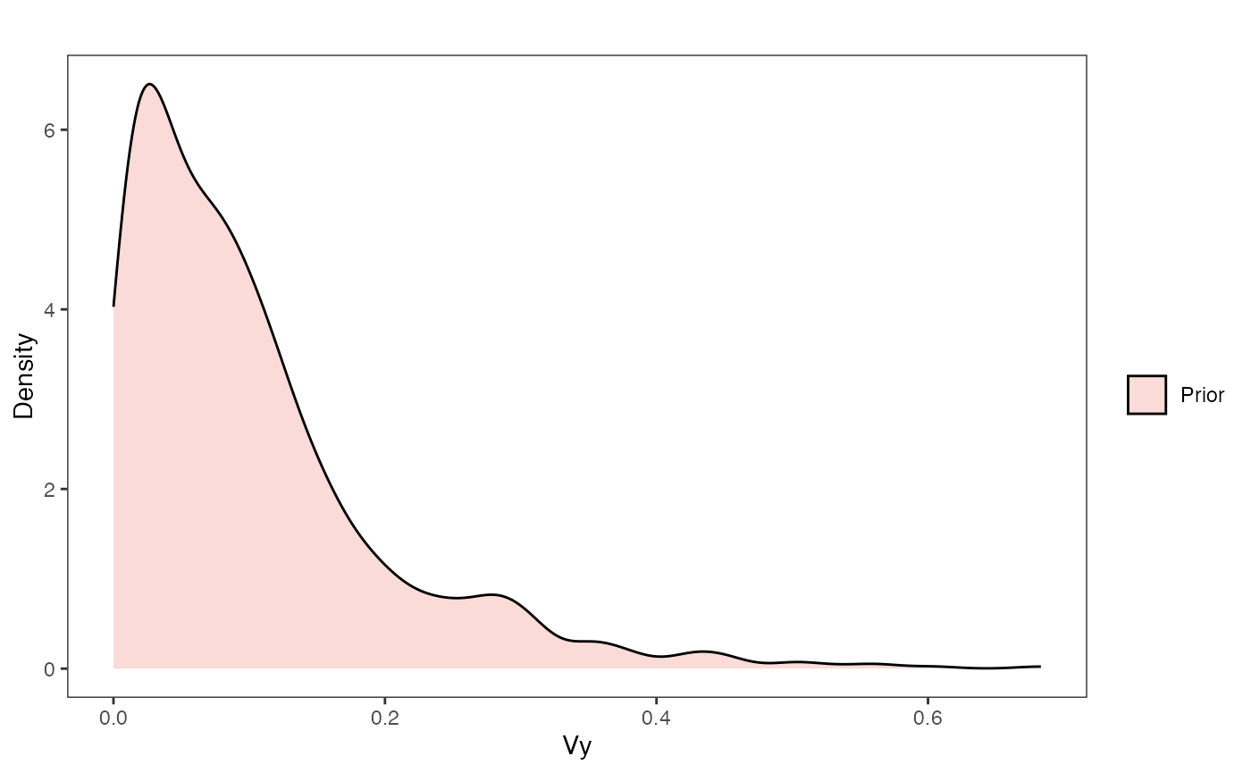

covariance.prior.direct.plot.code(hl.prior,vy.prior)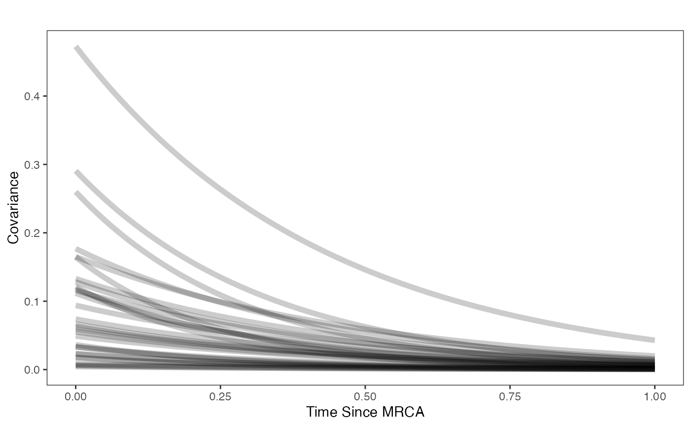

reg.direct.prior.plot.code(trdata,optima.prior,beta.prior)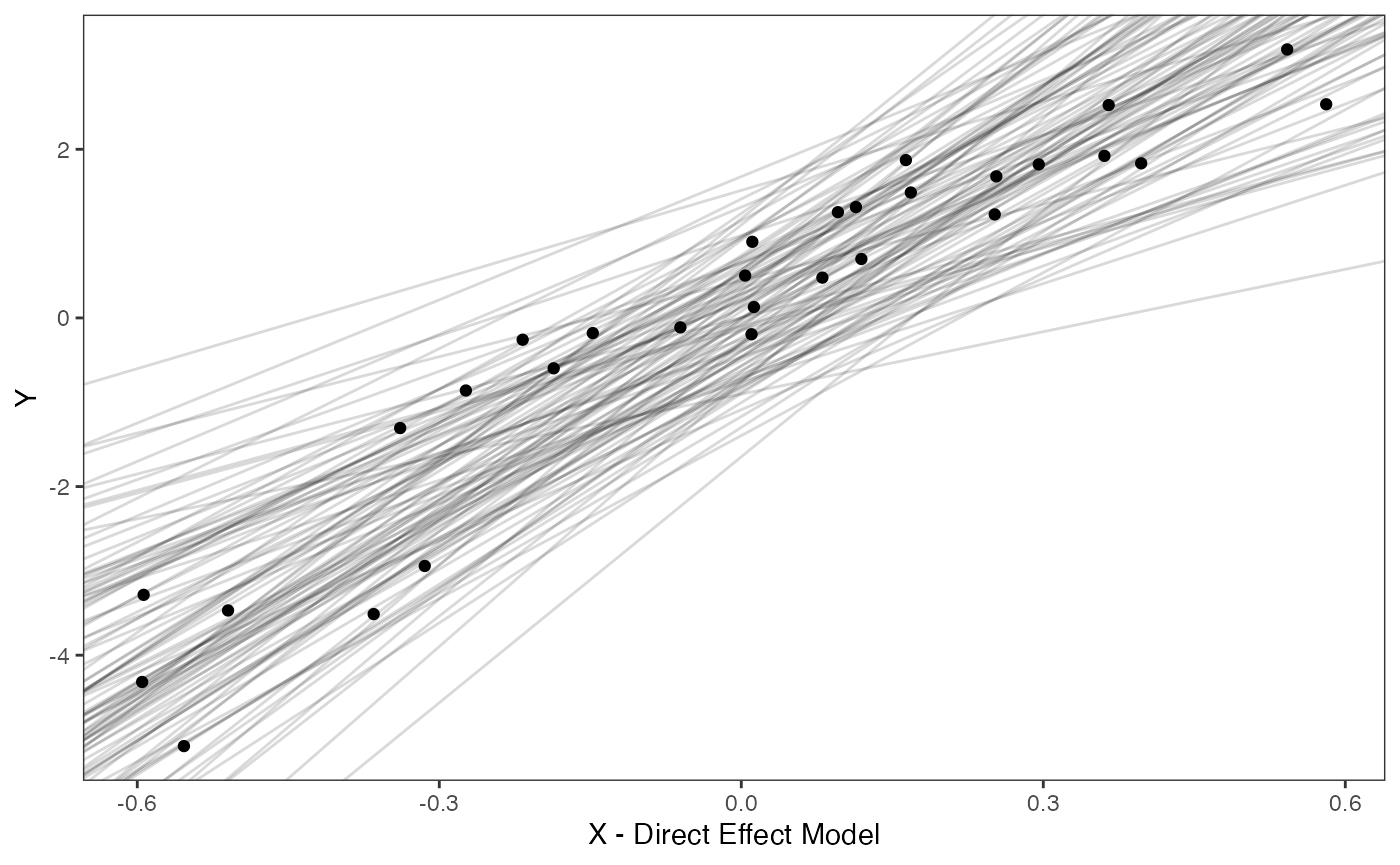

Data setup for Blouch

The line below combines the existing trdata file from make.trdata which has regime info for the tips with the X and Y values and their errors. We will use the helper function blouch.reg.direct.prep() to setup the dat object for Stan. This function and the other helper functions included with Blouch require trdata files, and then the names of the columns that contain Y and (sometimes depending on the model) X data and error data. “Z_direct” is the number of predictors, with “BGS” the name of the column where the tip regime data is located. The rest are the priors we defined above. See help info for each function and other articles on github.com for functionality.

dat<-blouch.reg.direct.prep(trdata,"Y_with_error","Y_error","X_with_error","X_error",Z_direct=1,"BGS",hl.prior,vy.prior,optima.prior,beta.prior)

Running models

First we will run the multi-optima direct effect model with varying intercepts. This will allow our intercepts (optima) to vary with the regimes, and these results will be similar to those from other OU model fitting approaches (e.g Slouch).

Now let’s run the model. Stan prints out a lot of info, so lets just look at the parameter estimates here and store the posterior distribution for later use.

#Combination of regime model with multiple traits direct effect model with measurement error and varying intercepts
fit.reg.direct<- rstan::sampling(object = blouch:::stanmodels$blouchOU_reg_direct,data = dat,chains = 2,cores=2,iter =4000)
#Fig S11 from Grabowski (in press)

Results

print(fit.reg.direct,pars = c("hl","vy","optima","beta"))
#> Inference for Stan model: blouchOU_reg_direct.
#> 2 chains, each with iter=4000; warmup=2000; thin=1; 
#> post-warmup draws per chain=2000, total post-warmup draws=4000.
#> 
#>            mean se_mean   sd  2.5%   25%   50%   75% 97.5% n_eff Rhat
#> hl         0.21    0.00 0.05  0.13  0.18  0.21  0.24  0.34  5957    1
#> vy         0.24    0.00 0.08  0.12  0.18  0.23  0.28  0.42  3444    1
#> optima[1] -1.01    0.01 0.35 -1.70 -1.24 -1.01 -0.78 -0.30  4814    1
#> optima[2]  0.23    0.00 0.20 -0.16  0.10  0.23  0.36  0.62  7651    1
#> optima[3]  0.46    0.00 0.22  0.00  0.31  0.46  0.60  0.87  5459    1
#> beta[1]    5.03    0.01 0.44  4.18  4.73  5.02  5.32  5.90  4589    1
#> 
#> Samples were drawn using NUTS(diag_e) at Tue Oct  8 13:42:04 2024.
#> For each parameter, n_eff is a crude measure of effective sample size,
#> and Rhat is the potential scale reduction factor on split chains (at 
#> convergence, Rhat=1).
post.basic<-rstan::extract(fit.reg.direct)
#Table S7 from Grabowski (in press)

Priors vs. posterior plots for multi-optima direct effect model

Half-life

########################################################################################################
#Composite Figures
post<-post.basic

mypal <- ggsci::pal_npg("nrc", alpha = 0.4)(2)
mypal[2]<-palette()[1]

hl.sims<-data.frame(rlnorm(n=1000,meanlog=hl.prior[1],sdlog=hl.prior[2]))
names(hl.sims)<-"prior.hl.sims"

hl.post<-data.frame(post$hl) #Using this model's posterior
names(hl.post)<-"post.hl.sims"
df<-data.frame(cbind(hl.sims,hl.post))

hl.plot<-ggplot2::ggplot(data=df)+
  ggplot2::geom_density(ggplot2::aes(prior.hl.sims, fill=mypal[2]),alpha=0.2)+
  ggplot2::geom_density(ggplot2::aes(post.hl.sims, fill=mypal[1]),alpha=0.2)+
  ggplot2::theme_bw()+
  ggplot2::theme(
    panel.grid.major = ggplot2::element_blank(),
    panel.grid.minor = ggplot2::element_blank())+
  ggplot2::labs(title="",x="Half-life", y = "Density")+
  #ggsci::scale_fill_npg(name="",labels=c("Posterior","Prior"))
  ggplot2::scale_fill_manual(values=mypal,name="",labels=c("Posterior","Prior"))

hl.plot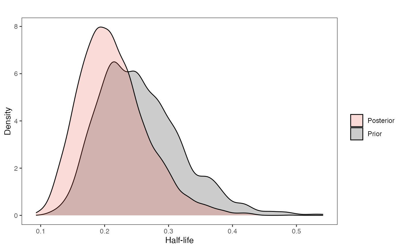

########################################################################################################
vy.sims<-rexp(n=1000,rate=vy.prior)
vy.sims<-data.frame(vy.sims)
names(vy.sims)<-"prior.vy.sims"

vy.post<-data.frame(post$vy)
names(vy.post)<-"post.vy.sims"

df<-data.frame(cbind(vy.sims,vy.post))

vy.plot<-ggplot2::ggplot(data=df)+
  ggplot2::geom_density(ggplot2::aes(prior.vy.sims, fill=mypal[2]),alpha=0.2)+
  ggplot2::geom_density(ggplot2::aes(post.vy.sims, fill=mypal[1]),alpha=0.2)+
  ggplot2::theme_bw()+
  ggplot2::theme(
    panel.grid.major = ggplot2::element_blank(),
    panel.grid.minor = ggplot2::element_blank())+
  ggplot2::labs(title="",x="Vy", y = "Density")+
  #ggsci::scale_fill_npg(name="",labels=c("Posterior","Prior"))
  ggplot2::scale_fill_manual(values=mypal,name="",labels=c("Posterior","Prior"))

vy.plot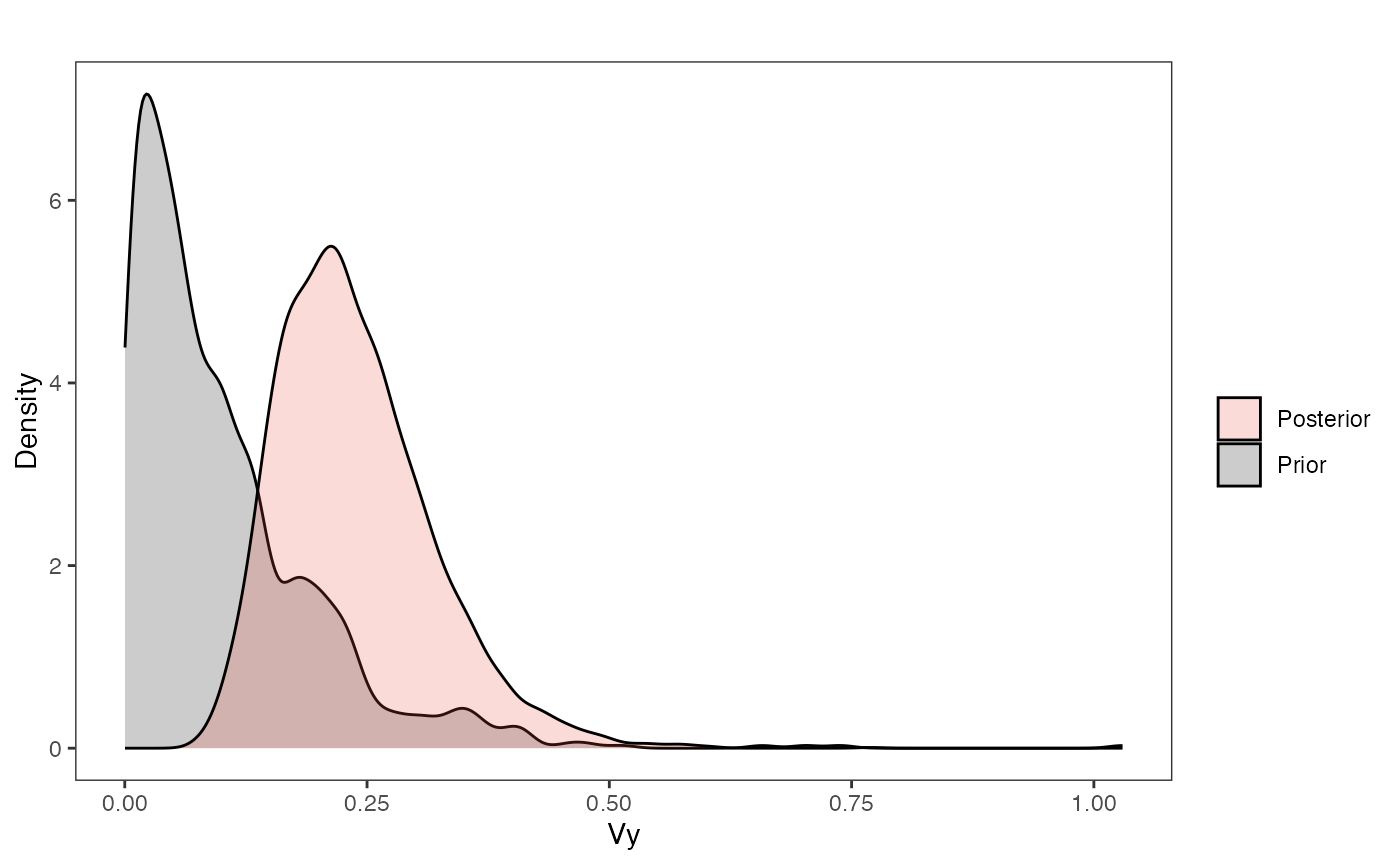

Covariance

########################################################################################################
hl.sims<-data.frame(rlnorm(n=1000,meanlog=hl.prior[1],sdlog=hl.prior[2]))
vy.sims<-rexp(n=1000,rate=vy.prior)
a.sims<-log(2)/hl.sims
sigma2_y.sims<-vy.sims*(2*(log(2)/hl.sims))
#mypal <- ggsci::pal_npg("nrc", alpha = 0.4)(2)
x<-seq(0,1,by=0.01)
df<-data.frame(x)
covariance.plot<-ggplot2::ggplot(df,ggplot2::aes(x))
for(i in 1:30){
  covariance.plot<-covariance.plot+ggplot2::stat_function(fun=function(x,i) {sigma2_y.sims[i,] /(2 * a.sims[i,]) * ((1 - exp(-2 * a.sims[i,] * (1-(x/2)))) * exp(-a.sims[i,] * x))},
                              args=list(i=i),alpha=0.2,lwd=2)
  covariance.plot<-covariance.plot+ggplot2::stat_function(fun=function(x,i) {post$sigma2_y[i] /(2 * post$a[i]) * ((1 - exp(-2 * post$a[i] * (1-(x/2)))) * exp(-post$a[i] * x))},
                              args=list(i=i),alpha=0.2,lwd=2,color=mypal[1])
}
covariance.plot<-covariance.plot+ggplot2::theme_bw()+
  ggplot2::theme(
    panel.grid.major = ggplot2::element_blank(),
    panel.grid.minor = ggplot2::element_blank())+
  ggplot2::labs(title="",x="Time Since MRCA", y = "Covariance")+
  ggplot2::scale_fill_manual(values=mypal,name="",labels=c("Prior","Posterior"))

covariance.plot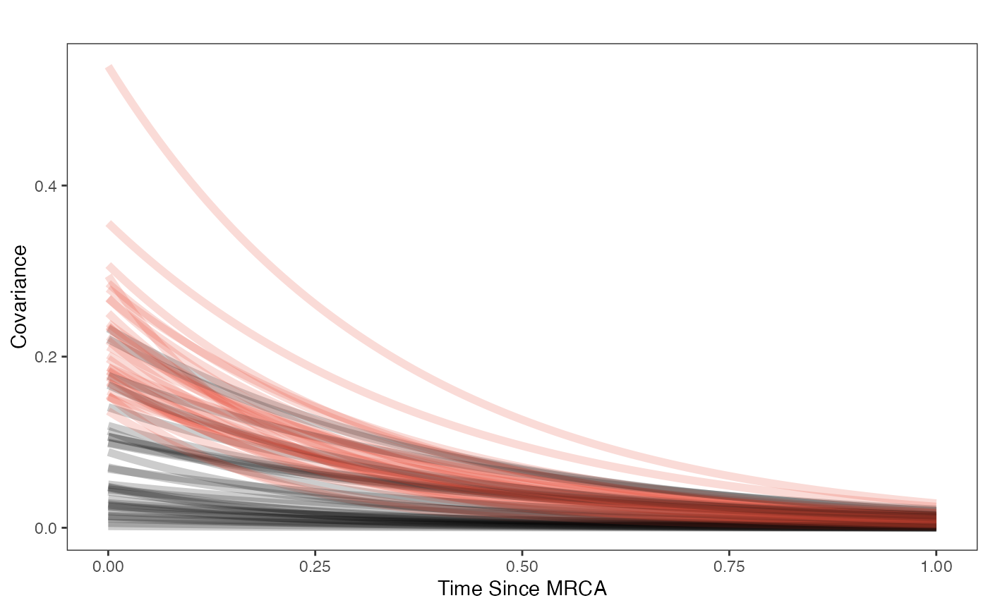

Regression plots

########################################################################################################
#Varying intercepts
post<-post.basic
mypal <- ggsci::pal_aaas("default", alpha = 1)(3)

optima.sims<-rnorm(100,optima.prior[1],optima.prior[2])
beta.sims<-rnorm(n=100,beta.prior[1],beta.prior[2])

optima.post<-post$optima
beta.post<-data.frame(post$beta)
names(beta.post)<-c("post.beta.1")


mu.link.11<-function(x.seq){optima.post[,1]+x.seq*beta.post[,1]}
mu.link.12<-function(x.seq){optima.post[,2]+x.seq*beta.post[,1]}
mu.link.13<-function(x.seq){optima.post[,3]+x.seq*beta.post[,1]}


x.seq <- seq(from=min(trdata$dat$X_with_error), to=max(trdata$dat$X_with_error) , length.out=100)
mu.11 <- sapply(x.seq , mu.link.11 )
mu.12 <- sapply(x.seq , mu.link.12 )
mu.13 <- sapply(x.seq , mu.link.13 )


mu.mean.11<-colMeans(mu.11)
mu.mean.12<-colMeans(mu.12)
mu.mean.13<-colMeans(mu.13)


mu.mean.11<-data.frame(as.numeric(mu.mean.11))
mu.mean.12<-data.frame(as.numeric(mu.mean.12))
mu.mean.13<-data.frame(as.numeric(mu.mean.13))

names(mu.mean.11)<-"mu.mean.11"
names(mu.mean.12)<-"mu.mean.12"
names(mu.mean.13)<-"mu.mean.13"


mu.CI.11 <- apply( mu.11 , MARGIN=2, FUN=rethinking::PI , prob=0.89 )
mu.CI.12 <- apply( mu.12 , MARGIN=2, FUN=rethinking::PI , prob=0.89 )
mu.CI.13 <- apply( mu.13 , MARGIN=2, FUN=rethinking::PI , prob=0.89 )


mu.CI.11<-data.frame(t(data.frame(mu.CI.11)),x.seq)
mu.CI.12<-data.frame(t(data.frame(mu.CI.12)),x.seq)
mu.CI.13<-data.frame(t(data.frame(mu.CI.13)),x.seq)


names(mu.CI.11)<-c("min.5.5","max.94.5","x.seq")
names(mu.CI.12)<-c("min.5.5","max.94.5","x.seq")
names(mu.CI.13)<-c("min.5.5","max.94.5","x.seq")

df<-data.frame(Y=trdata$dat$Y_with_error,X=trdata$dat$X_with_error,Regimes=trdata$dat$BGS)
df11<-data.frame(x.seq,mu.mean.11)
df12<-data.frame(x.seq,mu.mean.12)
df13<-data.frame(x.seq,mu.mean.13)

regression.plot<-ggplot2::ggplot()+  
  ggplot2::geom_point(data=df,ggplot2::aes(y=Y,x=X,color=as.factor(Regimes)))+
  ggplot2::geom_abline(intercept=optima.sims,slope=beta.sims,alpha=0.05)+ #Prior
  
  ggplot2::geom_ribbon(data=mu.CI.11,ggplot2::aes(x=x.seq,ymin=min.5.5,ymax=max.94.5),linetype=2,alpha=0.1)+
  ggplot2::geom_line(data=df11,ggplot2::aes(x=x.seq,y=mu.mean.11),linetype=1,linewidth=1,alpha=0.75,color=mypal[1])+
  ggplot2::geom_ribbon(data=mu.CI.12,ggplot2::aes(x=x.seq,ymin=min.5.5,ymax=max.94.5),linetype=2,alpha=0.1)+
  ggplot2::geom_line(data=df12,ggplot2::aes(x=x.seq,y=mu.mean.12),linetype=1,linewidth=1,alpha=0.75,color=mypal[2])+
  ggplot2::geom_ribbon(data=mu.CI.13,ggplot2::aes(x=x.seq,ymin=min.5.5,ymax=max.94.5),linetype=2,alpha=0.1)+
  ggplot2::geom_line(data=df13,ggplot2::aes(x=x.seq,y=mu.mean.13),linetype=1,linewidth=1,alpha=0.75,color=mypal[3])+
  
  ggplot2::theme_bw()+
  ggplot2::theme(
    panel.grid.major = ggplot2::element_blank(),
    panel.grid.minor = ggplot2::element_blank())+
  
  ggplot2::ylab("log Antler Volume (l)") + ggplot2::xlab("log Posterior Skull Length (cm)")+
  ggplot2::scale_color_manual(name="Breeding Group \nSize",values=mypal,labels=c('1-2', '3-5', '>5'))

regression.plot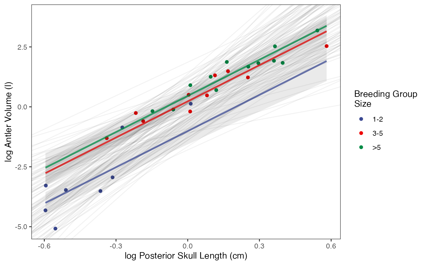

#Label points

Let’s combine all four plots into one plot

regression.plot<-regression.plot+ggplot2::theme(legend.position="none")
fig<-ggpubr::ggarrange(hl.plot, vy.plot,covariance.plot,regression.plot,ncol=2,nrow=2, labels = c("A)","B)","C)","D)"),common.legend = TRUE,legend="top")
#fig<-ggpubr::annotate_figure(fig,top=paste("Multi-Optima Adaptive Model - Varying Effects,\n hl=",hl,sep=""))
#ggplot2::ggsave("/Users/markgrabowski/Documents/Academic/Research/Current Projects/Blouch Project - SBR2/Blouch ms/R2/Figures/FigS11.pdf", plot = fig, width=7, height=7 )
fig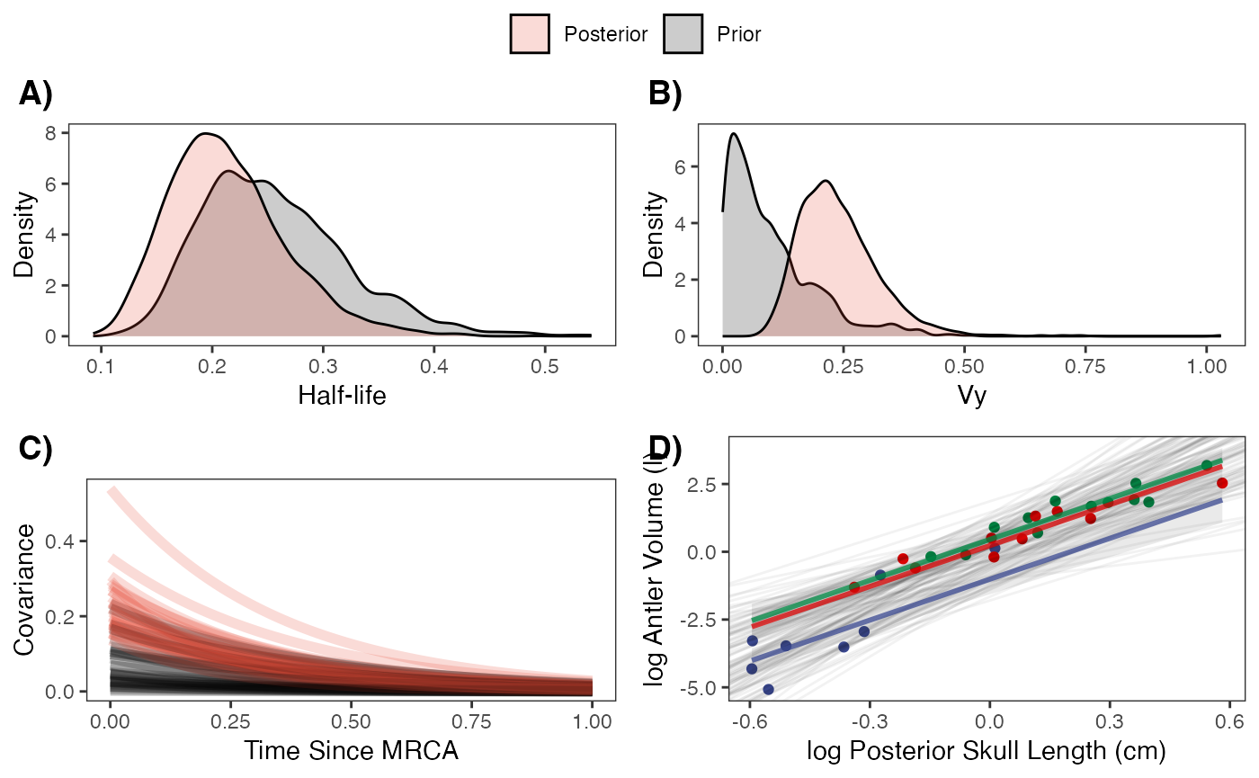

Multi-optima direct effect model with varying effects

Now lets run the multi-optima direct effect model with varying effects. This will allow our intercepts (optima) and slopes to vary with the regimes, but does not allow for multilevel modeling. We will use the same priors and the sane data formatting step above to produce our “dat” file.

fit.reg.direct.ve<- rstan::sampling(object = blouch:::stanmodels$blouchOU_reg_direct_ve,data = dat,chains = 2,cores=2,iter =4000)
#> Found more than one class "stanfit" in cache; using the first, from namespace 'rstan'
#> Also defined by 'rethinking'
#> Found more than one class "stanfit" in cache; using the first, from namespace 'rstan'
#> Also defined by 'rethinking'
#Fig S8 from Grabowski (in press)

Results

print(fit.reg.direct.ve,pars = c("hl","vy","optima","beta"))
#> Inference for Stan model: blouchOU_reg_direct_ve.
#> 2 chains, each with iter=4000; warmup=2000; thin=1; 
#> post-warmup draws per chain=2000, total post-warmup draws=4000.
#> 
#>           mean se_mean   sd  2.5%   25%  50%  75% 97.5% n_eff Rhat
#> hl        0.24    0.00 0.06  0.14  0.20 0.23 0.28  0.38  5976    1
#> vy        0.20    0.00 0.07  0.10  0.15 0.18 0.23  0.36  2521    1
#> optima[1] 0.17    0.01 0.53 -0.87 -0.20 0.17 0.52  1.23  3447    1
#> optima[2] 0.27    0.00 0.18 -0.08  0.15 0.27 0.38  0.64  5895    1
#> optima[3] 0.53    0.00 0.23  0.07  0.38 0.54 0.68  0.99  4472    1
#> beta[1,1] 7.27    0.01 0.84  5.69  6.68 7.27 7.83  8.92  3324    1
#> beta[2,1] 4.47    0.01 0.57  3.36  4.10 4.45 4.83  5.62  5696    1
#> beta[3,1] 4.62    0.01 0.59  3.48  4.22 4.59 5.02  5.84  3930    1
#> 
#> Samples were drawn using NUTS(diag_e) at Tue Oct  8 13:42:28 2024.
#> For each parameter, n_eff is a crude measure of effective sample size,
#> and Rhat is the potential scale reduction factor on split chains (at 
#> convergence, Rhat=1).
post.ve<-rstan::extract(fit.reg.direct.ve)

Priors vs. posterior plots for multi-optima direct effect model with varying effects

Lets look at the Prior versus Posterior plots of the parameter estimates

########################################################################################################
#Composite Figures
post<-post.ve

mypal <- ggsci::pal_npg("nrc", alpha = 0.4)(2)
mypal[2]<-palette()[1]

hl.sims<-data.frame(rlnorm(n=1000,meanlog=hl.prior[1],sdlog=hl.prior[2]))
names(hl.sims)<-"prior.hl.sims"

hl.post<-data.frame(post$hl) #Using this model's posterior
names(hl.post)<-"post.hl.sims"
df<-data.frame(cbind(hl.sims,hl.post))

hl.plot<-ggplot2::ggplot(data=df)+
  ggplot2::geom_density(ggplot2::aes(prior.hl.sims, fill=mypal[2]),alpha=0.2)+
  ggplot2::geom_density(ggplot2::aes(post.hl.sims, fill=mypal[1]),alpha=0.2)+
  ggplot2::theme_bw()+
  ggplot2::theme(
    panel.grid.major = ggplot2::element_blank(),
    panel.grid.minor = ggplot2::element_blank())+
  ggplot2::labs(title="",x="Half-life", y = "Density")+
  #ggsci::scale_fill_npg(name="",labels=c("Posterior","Prior"))
  ggplot2::scale_fill_manual(values=mypal,name="",labels=c("Posterior","Prior"))

hl.plot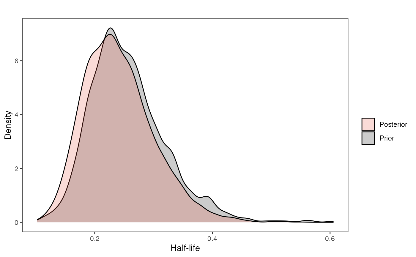

########################################################################################################
vy.sims<-rexp(n=1000,rate=vy.prior)
vy.sims<-data.frame(vy.sims)
names(vy.sims)<-"prior.vy.sims"

vy.post<-data.frame(post$vy)
names(vy.post)<-"post.vy.sims"

df<-data.frame(cbind(vy.sims,vy.post))

vy.plot<-ggplot2::ggplot(data=df)+
  ggplot2::geom_density(ggplot2::aes(prior.vy.sims, fill=mypal[2]),alpha=0.2)+
  ggplot2::geom_density(ggplot2::aes(post.vy.sims, fill=mypal[1]),alpha=0.2)+
  ggplot2::theme_bw()+
  ggplot2::theme(
    panel.grid.major = ggplot2::element_blank(),
    panel.grid.minor = ggplot2::element_blank())+
  ggplot2::labs(title="",x="Vy", y = "Density")+
  #ggsci::scale_fill_npg(name="",labels=c("Posterior","Prior"))
  ggplot2::scale_fill_manual(values=mypal,name="",labels=c("Posterior","Prior"))

vy.plot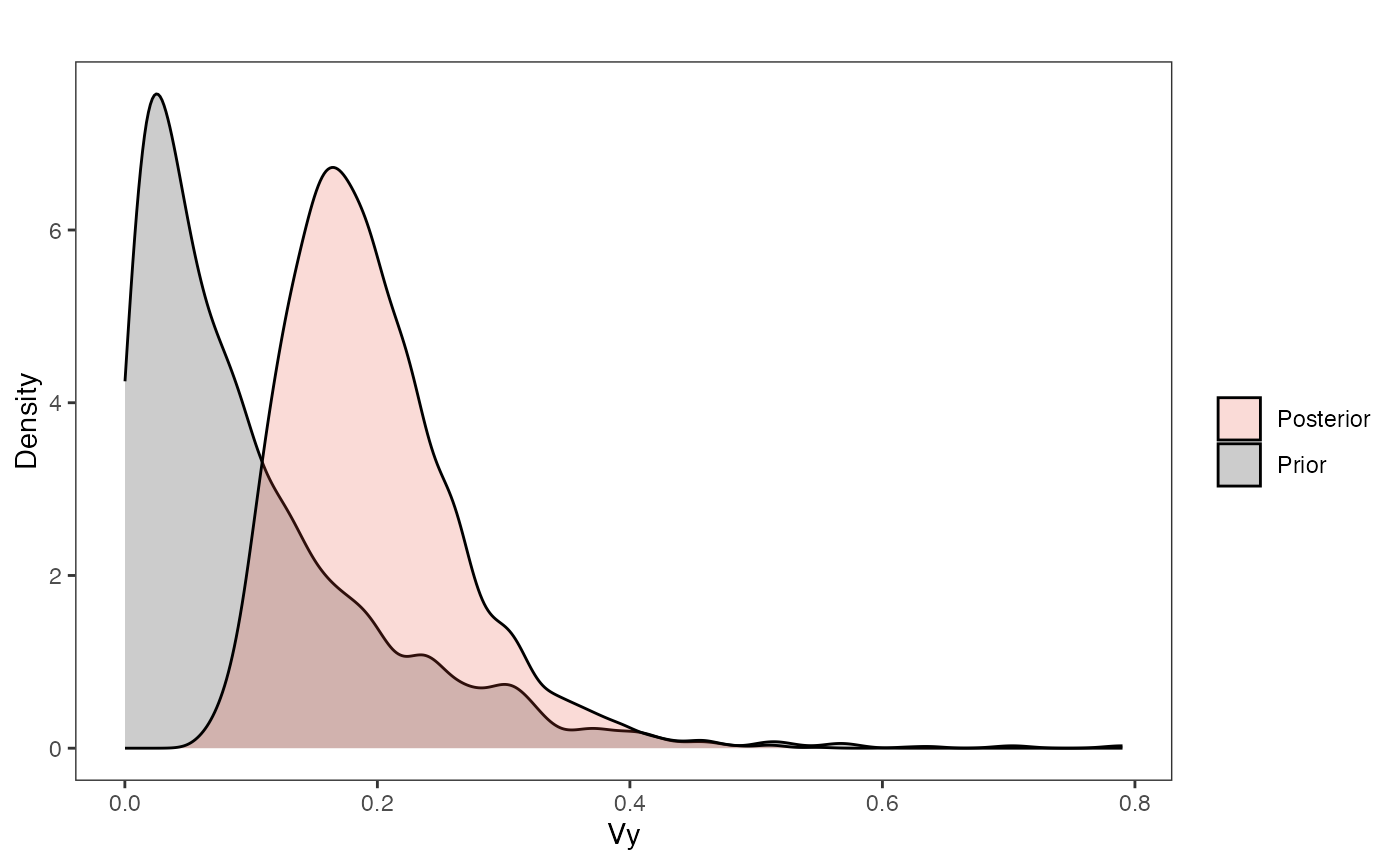

Covariance

########################################################################################################
hl.sims<-data.frame(rlnorm(n=1000,meanlog=hl.prior[1],sdlog=hl.prior[2]))
vy.sims<-rexp(n=1000,rate=vy.prior)
a.sims<-log(2)/hl.sims
sigma2_y.sims<-vy.sims*(2*(log(2)/hl.sims))
#mypal <- ggsci::pal_npg("nrc", alpha = 0.4)(2)
x<-seq(0,1,by=0.01)
df<-data.frame(x)
covariance.plot<-ggplot2::ggplot(df,ggplot2::aes(x))
for(i in 1:30){
  covariance.plot<-covariance.plot+ggplot2::stat_function(fun=function(x,i) {sigma2_y.sims[i,] /(2 * a.sims[i,]) * ((1 - exp(-2 * a.sims[i,] * (1-(x/2)))) * exp(-a.sims[i,] * x))},
                              args=list(i=i),alpha=0.2,lwd=2)
  covariance.plot<-covariance.plot+ggplot2::stat_function(fun=function(x,i) {post$sigma2_y[i] /(2 * post$a[i]) * ((1 - exp(-2 * post$a[i] * (1-(x/2)))) * exp(-post$a[i] * x))},
                              args=list(i=i),alpha=0.2,lwd=2,color=mypal[1])
}
covariance.plot<-covariance.plot+ggplot2::theme_bw()+
  ggplot2::theme(
    panel.grid.major = ggplot2::element_blank(),
    panel.grid.minor = ggplot2::element_blank())+
  ggplot2::labs(title="",x="Time Since MRCA", y = "Covariance")+
  ggplot2::scale_fill_manual(values=mypal,name="",labels=c("Prior","Posterior"))

covariance.plot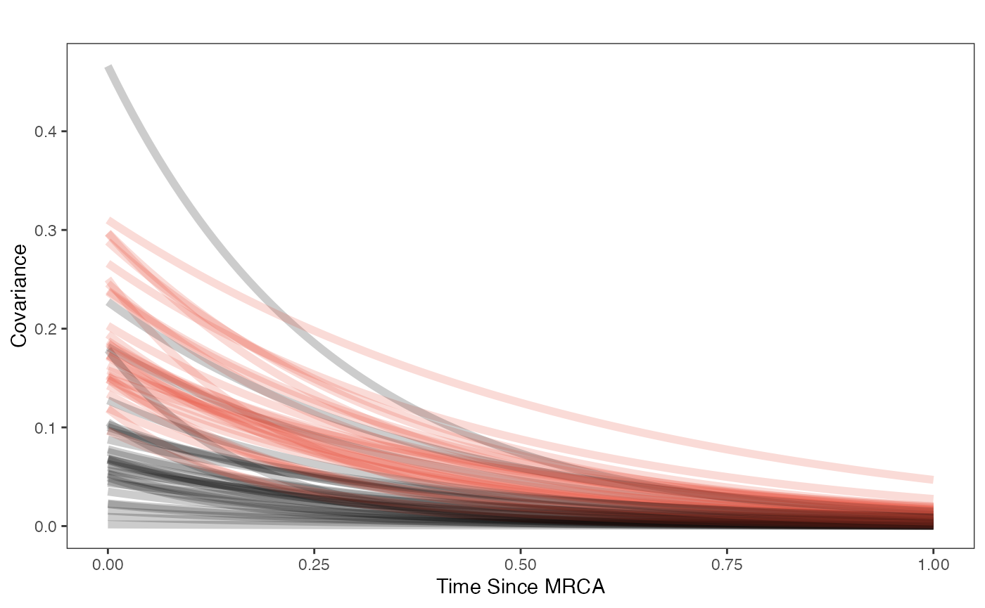

Now lets look at the varying effects model

########################################################################################################
#For Fig. 2
X<-dat$X_obs
Y<-dat$Y_obs

mypal <- ggsci::pal_aaas("default", alpha = 1)(3)

optima.sims<-rnorm(100,optima.prior[1],optima.prior[2])
beta.sims<-rnorm(n=100,beta.prior[1],beta.prior[2])

optima.post<-post$optima
beta.post<-data.frame(post$beta)
names(beta.post)<-c("post.beta.1","post.beta.2","post.beta.3")


mu.link.11<-function(x.seq){optima.post[,1]+x.seq*beta.post[,1]}
mu.link.12<-function(x.seq){optima.post[,2]+x.seq*beta.post[,2]}
mu.link.13<-function(x.seq){optima.post[,3]+x.seq*beta.post[,3]}


x.seq <- seq(from=min(X), to=max(X) , length.out=100)
mu.11 <- sapply(x.seq , mu.link.11 )
mu.12 <- sapply(x.seq , mu.link.12 )
mu.13 <- sapply(x.seq , mu.link.13 )


mu.mean.11<-colMeans(mu.11)
mu.mean.12<-colMeans(mu.12)
mu.mean.13<-colMeans(mu.13)


mu.mean.11<-data.frame(as.numeric(mu.mean.11))
mu.mean.12<-data.frame(as.numeric(mu.mean.12))
mu.mean.13<-data.frame(as.numeric(mu.mean.13))

names(mu.mean.11)<-"mu.mean.11"
names(mu.mean.12)<-"mu.mean.12"
names(mu.mean.13)<-"mu.mean.13"


mu.CI.11 <- apply( mu.11 , MARGIN=2, FUN=rethinking::PI , prob=0.89 )
mu.CI.12 <- apply( mu.12 , MARGIN=2, FUN=rethinking::PI , prob=0.89 )
mu.CI.13 <- apply( mu.13 , MARGIN=2, FUN=rethinking::PI , prob=0.89 )


mu.CI.11<-data.frame(t(data.frame(mu.CI.11)),x.seq)
mu.CI.12<-data.frame(t(data.frame(mu.CI.12)),x.seq)
mu.CI.13<-data.frame(t(data.frame(mu.CI.13)),x.seq)


names(mu.CI.11)<-c("min.5.5","max.94.5","x.seq")
names(mu.CI.12)<-c("min.5.5","max.94.5","x.seq")
names(mu.CI.13)<-c("min.5.5","max.94.5","x.seq")

#df<-data.frame(Y=stan_sim_data$Y,X=stan_sim_data$direct_cov)
df<-data.frame(Y=dat$Y_obs,X=dat$X_obs,Regimes=regimes_tip)
df11<-data.frame(x.seq,mu.mean.11)
df12<-data.frame(x.seq,mu.mean.12)
df13<-data.frame(x.seq,mu.mean.13)

#slope.prior.plot<-ggplot(data=reg.trdata$dat,aes(y=Sim1,x=X))+
fig2<-ggplot2::ggplot()+  
  ggplot2::geom_abline(intercept=optima.sims,slope=beta.sims,alpha=0.04)+ #Prior
  
  ggplot2::geom_ribbon(data=mu.CI.11,ggplot2::aes(x=x.seq,ymin=min.5.5,ymax=max.94.5),linetype=2,alpha=0.1)+
  ggplot2::geom_line(data=df11,ggplot2::aes(x=x.seq,y=mu.mean.11),linetype=1,linewidth=1,alpha=0.75,color=mypal[1])+
  ggplot2::geom_ribbon(data=mu.CI.12,ggplot2::aes(x=x.seq,ymin=min.5.5,ymax=max.94.5),linetype=2,alpha=0.1)+
  ggplot2::geom_line(data=df12,ggplot2::aes(x=x.seq,y=mu.mean.12),linetype=1,linewidth=1,alpha=0.75,color=mypal[2])+
  ggplot2::geom_ribbon(data=mu.CI.13,ggplot2::aes(x=x.seq,ymin=min.5.5,ymax=max.94.5),linetype=2,alpha=0.1)+
  ggplot2::geom_line(data=df13,ggplot2::aes(x=x.seq,y=mu.mean.13),linetype=1,linewidth=1,alpha=0.75,color=mypal[3])+
  ggplot2::geom_point(data=df,ggplot2::aes(y=Y,x=X,color=as.factor(Regimes)))+
  
  ggplot2::theme_bw()+
  ggplot2::theme(
    panel.grid.major = ggplot2::element_blank(),
    panel.grid.minor = ggplot2::element_blank())+
  
  ggplot2:: ylab("log Antler Volume (l)") + ggplot2::xlab("log Posterior Skull Length (cm)")+
  ggplot2::scale_color_manual(name="Breeding \nGroup Size",values=mypal,labels=c('1-2', '3-5', '>5'))

fig2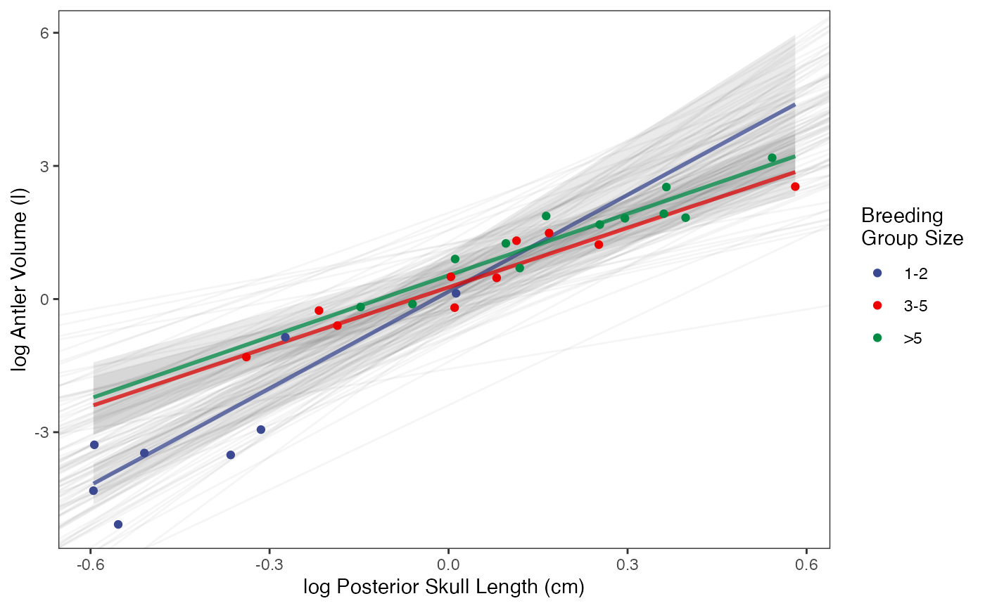


#ggplot2::ggsave("/Users/markgrabowski/Documents/Academic/Research/Current Projects/Blouch Project - SBR2/Blouch ms/R2/Figures/Fig2.pdf", plot = fig2, width=9, height=7 )

Let’s combine all four plots into one plot

fig2<-fig2+ggplot2::theme(legend.position="none")
fig<-ggpubr::ggarrange(hl.plot, vy.plot,covariance.plot,fig2,ncol=2,nrow=2, labels = c("A)","B)","C)","D)"),common.legend = TRUE,legend="top")
#ggplot2::ggsave("/Users/markgrabowski/Documents/Academic/Research/Current Projects/Blouch Project - SBR2/Blouch ms/R2/Figures/FigS8.pdf", plot = fig, width=7, height=7 )
fig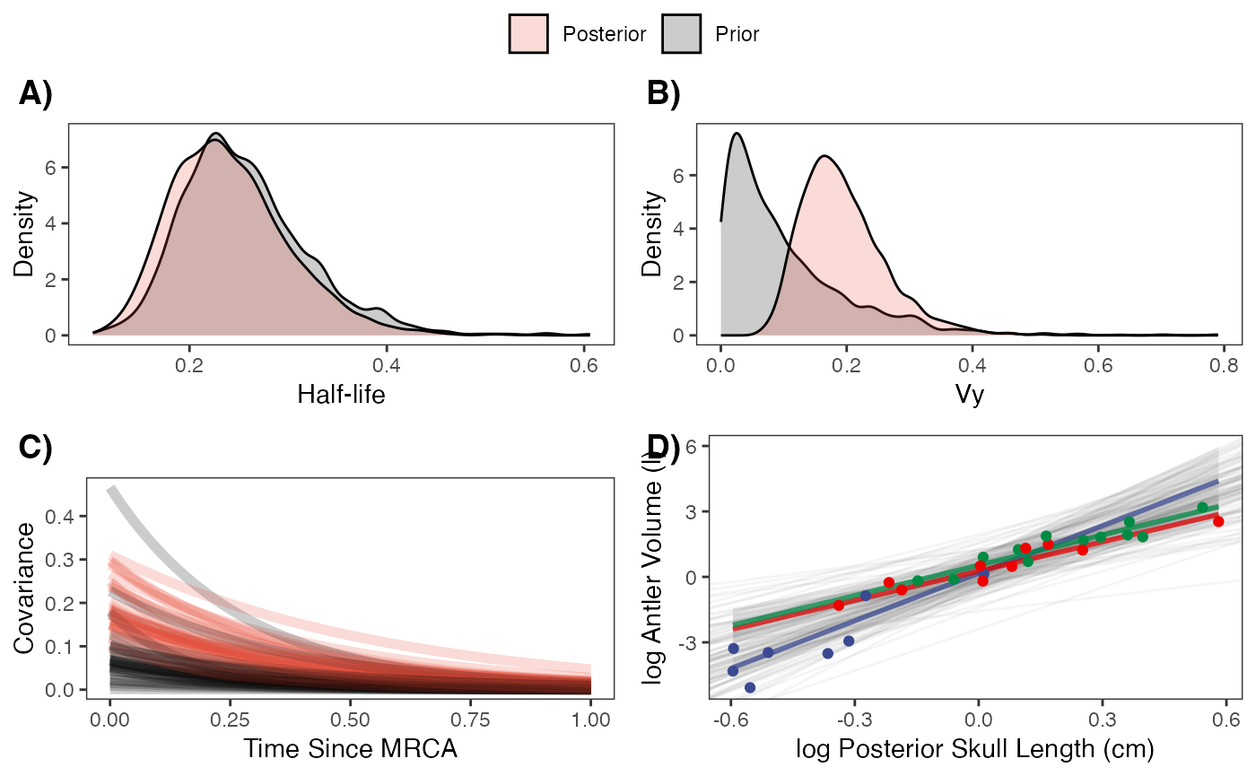

Multilevel Models

Now let’s run the multilevel version of those two models. As a multilevel model, information can be shared across the regimes, which can produce more accurate parameter estimates. Below are the priors used for this simulation. Here we use the non-centered version to aid in ease of calculation. See Grabowski (in press) for more on non-centered models. We will compare these all models in terms of their predictive performance at the end.

Below are the priors used for this first analysis. See Grabowski (in press) for more on setting these priors. The only new prior is on sigma

############################################################################################################
#Set Priors
hl.prior<-c(log(0.25),0.25)
vy.prior<-10
optima.prior<-c(0.05,0.75) #Informed by linear model
beta.prior<-c(6.304451,1.75) #Informed by linear model
sigma.prior<-c(0,1)

Multilevel Multi-Optima Direct Effect Model with Varying Intercepts

First we will run the multilevel multi-optima direct effect model with varying intercepts, which is non-centered for ease of estimation.

dat<-blouch.reg.direct.mlm.prep(trdata,"Y_with_error","Y_error","X_with_error","X_error",Z_direct=1,"BGS",hl.prior,vy.prior,optima.prior,beta.prior,sigma.prior)

Fit the model

fit.reg.direct.mlm.vi.nc<- rstan::sampling(object = blouch:::stanmodels$blouchOU_reg_direct_mlm_vi_nc,data = dat,chains = 2,cores=2,iter =4000,control = list(adapt_delta = 0.99))
#> Found more than one class "stanfit" in cache; using the first, from namespace 'rstan'
#> Also defined by 'rethinking'
#> Found more than one class "stanfit" in cache; using the first, from namespace 'rstan'
#> Also defined by 'rethinking'

#Fig S10/Table S6 in Grabowski (in press)

Let’s check out the results

print(fit.reg.direct.mlm.vi.nc,pars = c("hl","vy","optima","optima_bar","beta","sigma"))
#> Inference for Stan model: blouchOU_reg_direct_mlm_vi_nc.
#> 2 chains, each with iter=4000; warmup=2000; thin=1; 
#> post-warmup draws per chain=2000, total post-warmup draws=4000.
#> 
#>             mean se_mean   sd  2.5%   25%   50%   75% 97.5% n_eff Rhat
#> hl          0.22    0.00 0.05  0.13  0.18  0.21  0.25  0.34  3541    1
#> vy          0.24    0.00 0.08  0.12  0.18  0.23  0.28  0.42  2087    1
#> optima[1]  -1.02    0.01 0.44 -1.87 -1.31 -1.03 -0.74 -0.12  1942    1
#> optima[2]   0.23    0.00 0.19 -0.16  0.10  0.23  0.35  0.60  4080    1
#> optima[3]   0.45    0.00 0.23 -0.02  0.30  0.45  0.60  0.89  2741    1
#> optima_bar -0.08    0.01 0.43 -0.94 -0.34 -0.07  0.19  0.78  1483    1
#> beta[1]     5.02    0.01 0.48  4.12  4.70  5.00  5.33  6.02  1717    1
#> sigma       0.92    0.01 0.43  0.25  0.61  0.85  1.15  1.93  1766    1
#> 
#> Samples were drawn using NUTS(diag_e) at Tue Oct  8 13:43:36 2024.
#> For each parameter, n_eff is a crude measure of effective sample size,
#> and Rhat is the potential scale reduction factor on split chains (at 
#> convergence, Rhat=1).
post.mlm.vi<-rstan::extract(fit.reg.direct.mlm.vi.nc)

Priors vs. posterior plots for multilevel multi-optima direct effect model with varying intercepts

Lets look at the Prior versus Posterior plots of the parameter estimates Half-life

########################################################################################################
#Composite Figures
post<-post.mlm.vi

mypal <- ggsci::pal_npg("nrc", alpha = 0.4)(2)
mypal[2]<-palette()[1]

hl.sims<-data.frame(rlnorm(n=1000,meanlog=hl.prior[1],sdlog=hl.prior[2]))
names(hl.sims)<-"prior.hl.sims"

hl.post<-data.frame(post$hl) #Using this model's posterior
names(hl.post)<-"post.hl.sims"
df<-data.frame(cbind(hl.sims,hl.post))

hl.plot<-ggplot2::ggplot(data=df)+
  ggplot2::geom_density(ggplot2::aes(prior.hl.sims, fill=mypal[2]),alpha=0.2)+
  ggplot2::geom_density(ggplot2::aes(post.hl.sims, fill=mypal[1]),alpha=0.2)+
  ggplot2::theme_bw()+
  ggplot2::theme(
    panel.grid.major = ggplot2::element_blank(),
    panel.grid.minor = ggplot2::element_blank())+
  ggplot2::labs(title="",x="Half-life", y = "Density")+
  #ggsci::scale_fill_npg(name="",labels=c("Posterior","Prior"))
  ggplot2::scale_fill_manual(values=mypal,name="",labels=c("Posterior","Prior"))

hl.plot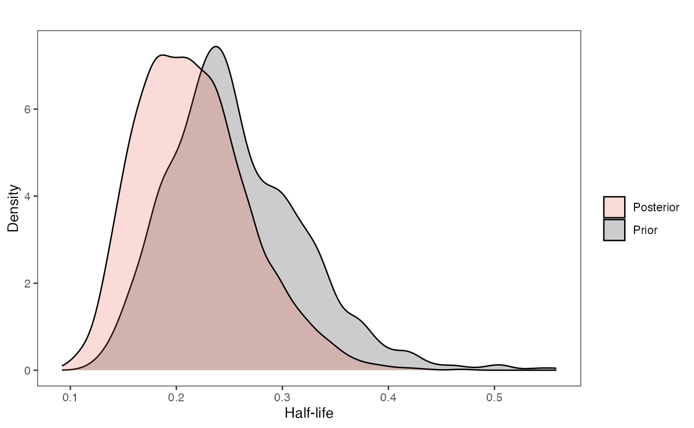

########################################################################################################
vy.sims<-rexp(n=1000,rate=vy.prior)
vy.sims<-data.frame(vy.sims)
names(vy.sims)<-"prior.vy.sims"

vy.post<-data.frame(post$vy)
names(vy.post)<-"post.vy.sims"

df<-data.frame(cbind(vy.sims,vy.post))

vy.plot<-ggplot2::ggplot(data=df)+
  ggplot2::geom_density(ggplot2::aes(prior.vy.sims, fill=mypal[2]),alpha=0.2)+
  ggplot2::geom_density(ggplot2::aes(post.vy.sims, fill=mypal[1]),alpha=0.2)+
  ggplot2::theme_bw()+
  ggplot2::theme(
    panel.grid.major = ggplot2::element_blank(),
    panel.grid.minor = ggplot2::element_blank())+
  ggplot2::labs(title="",x="Vy", y = "Density")+
  #ggsci::scale_fill_npg(name="",labels=c("Posterior","Prior"))
  ggplot2::scale_fill_manual(values=mypal,name="",labels=c("Posterior","Prior"))

vy.plot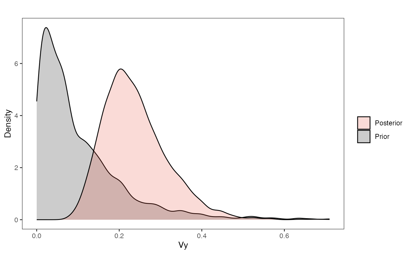

Covariance

########################################################################################################
hl.sims<-data.frame(rlnorm(n=1000,meanlog=hl.prior[1],sdlog=hl.prior[2]))
vy.sims<-rexp(n=1000,rate=vy.prior)
a.sims<-log(2)/hl.sims
sigma2_y.sims<-vy.sims*(2*(log(2)/hl.sims))
#mypal <- ggsci::pal_npg("nrc", alpha = 0.4)(2)
x<-seq(0,1,by=0.01)
df<-data.frame(x)
covariance.plot<-ggplot2::ggplot(df,ggplot2::aes(x))
for(i in 1:30){
  covariance.plot<-covariance.plot+ggplot2::stat_function(fun=function(x,i) {sigma2_y.sims[i,] /(2 * a.sims[i,]) * ((1 - exp(-2 * a.sims[i,] * (1-(x/2)))) * exp(-a.sims[i,] * x))},
                              args=list(i=i),alpha=0.2,lwd=2)
  covariance.plot<-covariance.plot+ggplot2::stat_function(fun=function(x,i) {post$sigma2_y[i] /(2 * post$a[i]) * ((1 - exp(-2 * post$a[i] * (1-(x/2)))) * exp(-post$a[i] * x))},
                              args=list(i=i),alpha=0.2,lwd=2,color=mypal[1])
}
covariance.plot<-covariance.plot+ggplot2::theme_bw()+
  ggplot2::theme(
    panel.grid.major = ggplot2::element_blank(),
    panel.grid.minor = ggplot2::element_blank())+
  ggplot2::labs(title="",x="Time Since MRCA", y = "Covariance")+
  ggplot2::scale_fill_manual(values=mypal,name="",labels=c("Prior","Posterior"))

covariance.plot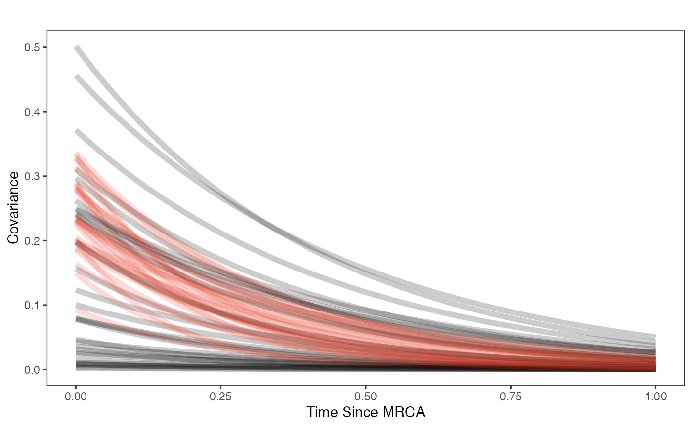

Regression Plots

########################################################################################################
#Varying intercepts
mypal <- ggsci::pal_aaas("default", alpha = 1)(3)

optima.sims<-rnorm(100,optima.prior[1],optima.prior[2])
beta.sims<-rnorm(n=100,beta.prior[1],beta.prior[2])

optima.post<-post$optima
beta.post<-data.frame(post$beta)
names(beta.post)<-c("post.beta.1")


mu.link.11<-function(x.seq){optima.post[,1]+x.seq*beta.post[,1]}
mu.link.12<-function(x.seq){optima.post[,2]+x.seq*beta.post[,1]}
mu.link.13<-function(x.seq){optima.post[,3]+x.seq*beta.post[,1]}


x.seq <- seq(from=min(trdata$dat$X_with_error), to=max(trdata$dat$X_with_error) , length.out=100)
mu.11 <- sapply(x.seq , mu.link.11 )
mu.12 <- sapply(x.seq , mu.link.12 )
mu.13 <- sapply(x.seq , mu.link.13 )


mu.mean.11<-colMeans(mu.11)
mu.mean.12<-colMeans(mu.12)
mu.mean.13<-colMeans(mu.13)


mu.mean.11<-data.frame(as.numeric(mu.mean.11))
mu.mean.12<-data.frame(as.numeric(mu.mean.12))
mu.mean.13<-data.frame(as.numeric(mu.mean.13))

names(mu.mean.11)<-"mu.mean.11"
names(mu.mean.12)<-"mu.mean.12"
names(mu.mean.13)<-"mu.mean.13"


mu.CI.11 <- apply( mu.11 , MARGIN=2, FUN=rethinking::PI , prob=0.89 )
mu.CI.12 <- apply( mu.12 , MARGIN=2, FUN=rethinking::PI , prob=0.89 )
mu.CI.13 <- apply( mu.13 , MARGIN=2, FUN=rethinking::PI , prob=0.89 )


mu.CI.11<-data.frame(t(data.frame(mu.CI.11)),x.seq)
mu.CI.12<-data.frame(t(data.frame(mu.CI.12)),x.seq)
mu.CI.13<-data.frame(t(data.frame(mu.CI.13)),x.seq)


names(mu.CI.11)<-c("min.5.5","max.94.5","x.seq")
names(mu.CI.12)<-c("min.5.5","max.94.5","x.seq")
names(mu.CI.13)<-c("min.5.5","max.94.5","x.seq")

df<-data.frame(Y=trdata$dat$Y_with_error,X=trdata$dat$X_with_error,Regimes=trdata$dat$BGS)
df11<-data.frame(x.seq,mu.mean.11)
df12<-data.frame(x.seq,mu.mean.12)
df13<-data.frame(x.seq,mu.mean.13)

regression.plot<-ggplot2::ggplot()+  
  ggplot2::geom_point(data=df,ggplot2::aes(y=Y,x=X,color=as.factor(Regimes)))+
  ggplot2::geom_abline(intercept=optima.sims,slope=beta.sims,alpha=0.05)+ #Prior
  
  ggplot2::geom_ribbon(data=mu.CI.11,ggplot2::aes(x=x.seq,ymin=min.5.5,ymax=max.94.5),linetype=2,alpha=0.1)+
  ggplot2::geom_line(data=df11,ggplot2::aes(x=x.seq,y=mu.mean.11),linetype=1,linewidth=1,alpha=0.75,color=mypal[1])+
  ggplot2::geom_ribbon(data=mu.CI.12,ggplot2::aes(x=x.seq,ymin=min.5.5,ymax=max.94.5),linetype=2,alpha=0.1)+
  ggplot2::geom_line(data=df12,ggplot2::aes(x=x.seq,y=mu.mean.12),linetype=1,linewidth=1,alpha=0.75,color=mypal[2])+
  ggplot2::geom_ribbon(data=mu.CI.13,ggplot2::aes(x=x.seq,ymin=min.5.5,ymax=max.94.5),linetype=2,alpha=0.1)+
  ggplot2::geom_line(data=df13,ggplot2::aes(x=x.seq,y=mu.mean.13),linetype=1,linewidth=1,alpha=0.75,color=mypal[3])+
  
  ggplot2::theme_bw()+
  ggplot2::theme(
    panel.grid.major = ggplot2::element_blank(),
    panel.grid.minor = ggplot2::element_blank())+
  
  ggplot2::ylab("log Antler Volume (l)") + ggplot2::xlab("log Posterior Skull Length (cm)")+
  ggplot2::scale_color_manual(name="Breeding Group \nSize",values=mypal,labels=c('1-2', '3-5', '>5'))

regression.plot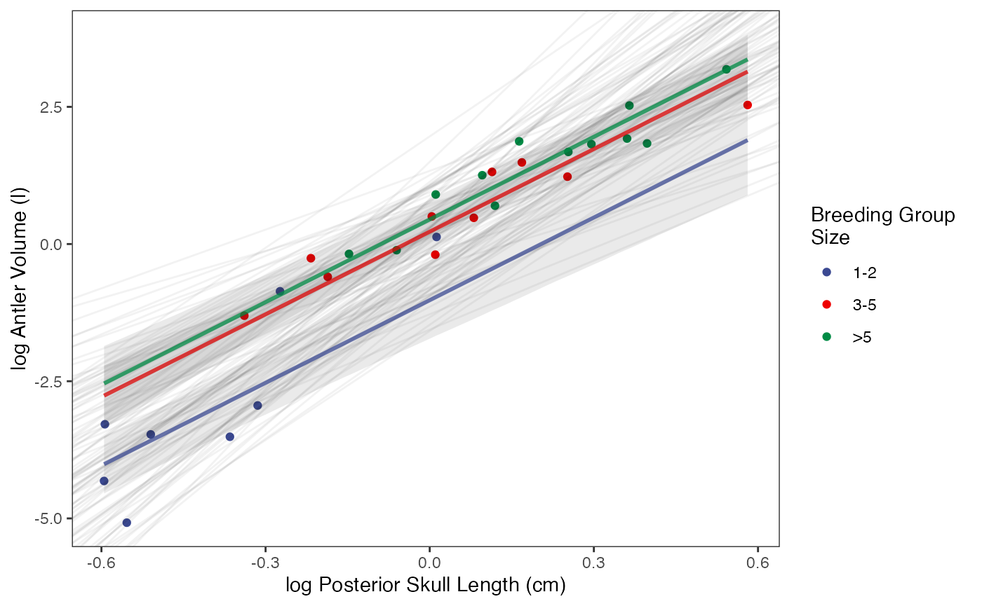

#Label points

Let’s combine all four plots into one plot

fig2<-fig2+ggplot2::theme(legend.position="none")
fig<-ggpubr::ggarrange(hl.plot, vy.plot,covariance.plot,regression.plot,ncol=2,nrow=2, labels = c("A)","B)","C)","D)"),common.legend = TRUE,legend="top")
#ggplot2::ggsave("/Users/markgrabowski/Documents/Academic/Research/Current Projects/Blouch Project - SBR2/Blouch ms/R2/Figures/FigS10.pdf", plot = fig, width=7, height=7 )
fig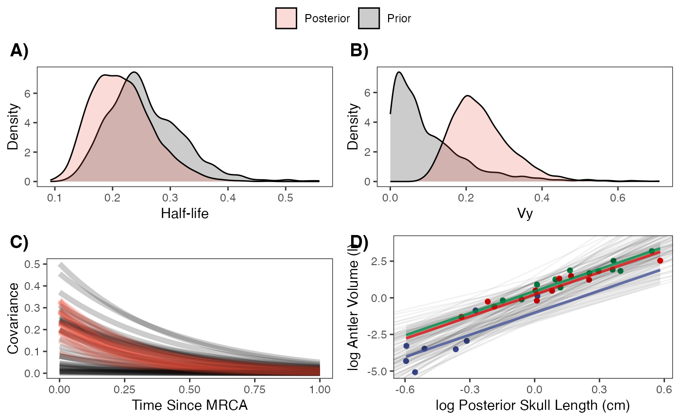

Multilevel Multi-Optima Direct Effect Model with Varying Effects

Now let’s run the Multilevel Multi-optima Direct Effect Model with Varying Effects. This will allow our intercepts (optima) and slopes to vary with the regimes. As a multilevel model, information can be shared across the regimes, which can produce more accurate parameter estimates.

fit.reg.direct.mlm.ve.nc<- rstan::sampling(object = blouch:::stanmodels$blouchOU_reg_direct_mlm_ve_nc,data = dat,chains = 2,cores=2,iter =4000,control = list(adapt_delta = 0.99))
#> Found more than one class "stanfit" in cache; using the first, from namespace 'rstan'
#> Also defined by 'rethinking'
#> Found more than one class "stanfit" in cache; using the first, from namespace 'rstan'
#> Also defined by 'rethinking'

Results

print(fit.reg.direct.mlm.ve.nc,pars = c("hl","vy","optima_bar","beta_bar","Rho[1,2]","sigma","optima","beta"))
#> Inference for Stan model: blouchOU_reg_direct_mlm_ve_nc.
#> 2 chains, each with iter=4000; warmup=2000; thin=1; 
#> post-warmup draws per chain=2000, total post-warmup draws=4000.
#> 
#>             mean se_mean   sd  2.5%   25%   50%  75% 97.5% n_eff Rhat
#> hl          0.24    0.00 0.06  0.14  0.20  0.23 0.27  0.38  5017    1
#> vy          0.20    0.00 0.07  0.10  0.15  0.19 0.24  0.36  2466    1
#> optima_bar  0.26    0.01 0.33 -0.52  0.10  0.29 0.46  0.84  1758    1
#> beta_bar    5.56    0.02 0.82  4.05  5.01  5.54 6.08  7.30  2413    1
#> Rho[1,2]   -0.06    0.00 0.32 -0.65 -0.29 -0.06 0.18  0.56  4283    1
#> sigma[1]    0.45    0.01 0.38  0.01  0.16  0.36 0.65  1.41  2036    1
#> sigma[2]    1.31    0.01 0.54  0.31  0.95  1.28 1.63  2.47  2152    1
#> optima[1]   0.09    0.01 0.52 -1.15 -0.17  0.18 0.42  0.97  1605    1
#> optima[2]   0.29    0.00 0.17 -0.07  0.18  0.29 0.41  0.62  4766    1
#> optima[3]   0.48    0.00 0.22  0.07  0.33  0.47 0.61  0.92  3810    1
#> beta[1,1]   7.00    0.02 0.88  5.06  6.50  7.07 7.58  8.56  1635    1
#> beta[2,1]   4.52    0.01 0.57  3.41  4.13  4.51 4.90  5.66  3294    1
#> beta[3,1]   4.74    0.01 0.59  3.57  4.36  4.74 5.13  5.86  4588    1
#> 
#> Samples were drawn using NUTS(diag_e) at Tue Oct  8 13:45:04 2024.
#> For each parameter, n_eff is a crude measure of effective sample size,
#> and Rhat is the potential scale reduction factor on split chains (at 
#> convergence, Rhat=1).
post.mlm.ve<-rstan::extract(fit.reg.direct.mlm.ve.nc)

Priors vs. posterior plots for multilevel multi-optima direct effect model with varying effects

Lets look at the Prior versus Posterior plots of the parameter estimates Half-life

########################################################################################################
#Composite Figures
post<-post.mlm.ve

mypal <- ggsci::pal_npg("nrc", alpha = 0.4)(2)
mypal[2]<-palette()[1]

hl.sims<-data.frame(rlnorm(n=1000,meanlog=hl.prior[1],sdlog=hl.prior[2]))
names(hl.sims)<-"prior.hl.sims"

hl.post<-data.frame(post$hl) #Using this model's posterior
names(hl.post)<-"post.hl.sims"
df<-data.frame(cbind(hl.sims,hl.post))

hl.plot<-ggplot2::ggplot(data=df)+
  ggplot2::geom_density(ggplot2::aes(prior.hl.sims, fill=mypal[2]),alpha=0.2)+
  ggplot2::geom_density(ggplot2::aes(post.hl.sims, fill=mypal[1]),alpha=0.2)+
  ggplot2::theme_bw()+
  ggplot2::theme(
    panel.grid.major = ggplot2::element_blank(),
    panel.grid.minor = ggplot2::element_blank())+
  ggplot2::labs(title="",x="Half-life", y = "Density")+
  #ggsci::scale_fill_npg(name="",labels=c("Posterior","Prior"))
  ggplot2::scale_fill_manual(values=mypal,name="",labels=c("Posterior","Prior"))

hl.plot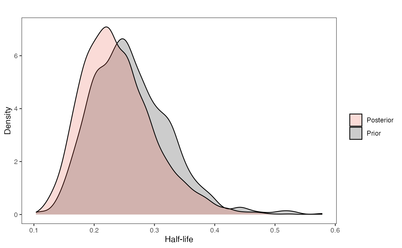

########################################################################################################
vy.sims<-rexp(n=1000,rate=vy.prior)
vy.sims<-data.frame(vy.sims)
names(vy.sims)<-"prior.vy.sims"

vy.post<-data.frame(post$vy)
names(vy.post)<-"post.vy.sims"

df<-data.frame(cbind(vy.sims,vy.post))

vy.plot<-ggplot2::ggplot(data=df)+
  ggplot2::geom_density(ggplot2::aes(prior.vy.sims, fill=mypal[2]),alpha=0.2)+
  ggplot2::geom_density(ggplot2::aes(post.vy.sims, fill=mypal[1]),alpha=0.2)+
  ggplot2::theme_bw()+
  ggplot2::theme(
    panel.grid.major = ggplot2::element_blank(),
    panel.grid.minor = ggplot2::element_blank())+
  ggplot2::labs(title="",x="Vy", y = "Density")+
  #ggsci::scale_fill_npg(name="",labels=c("Posterior","Prior"))
  ggplot2::scale_fill_manual(values=mypal,name="",labels=c("Posterior","Prior"))

vy.plot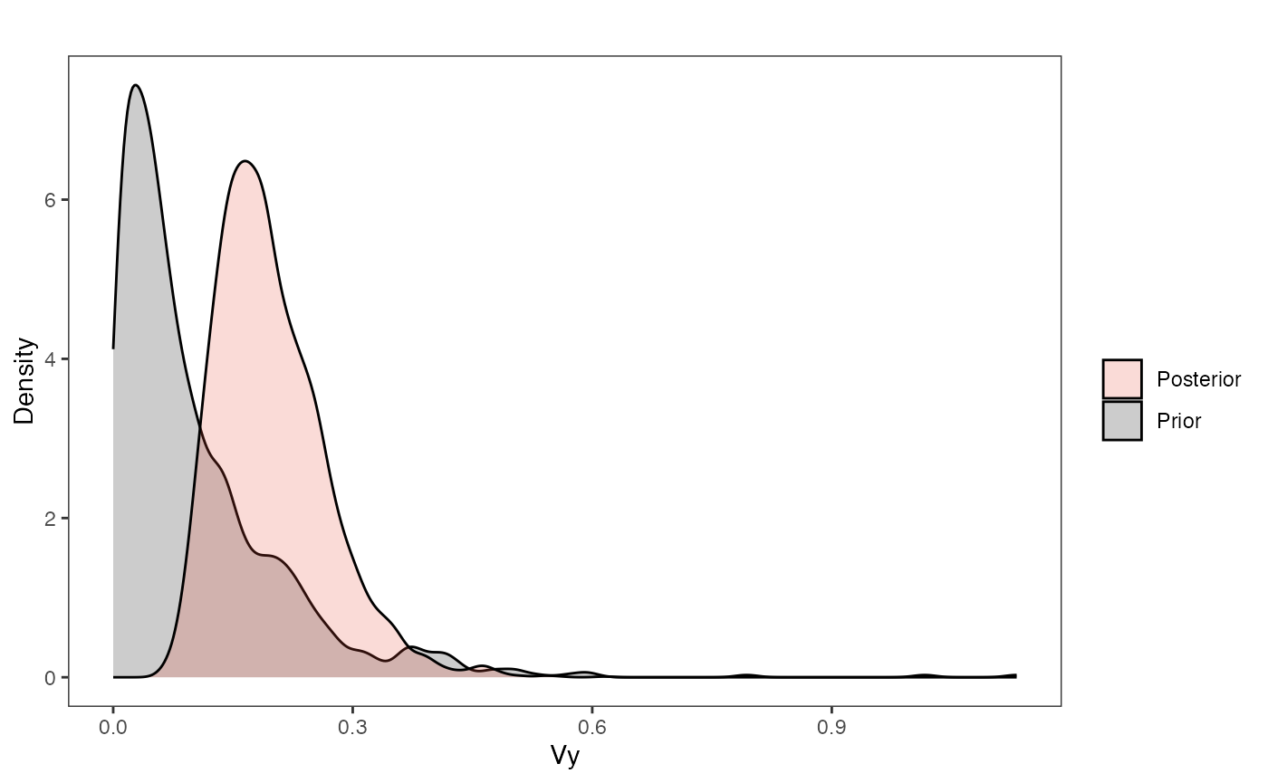

Covariance

########################################################################################################
hl.sims<-data.frame(rlnorm(n=1000,meanlog=hl.prior[1],sdlog=hl.prior[2]))
vy.sims<-rexp(n=1000,rate=vy.prior)
a.sims<-log(2)/hl.sims
sigma2_y.sims<-vy.sims*(2*(log(2)/hl.sims))
#mypal <- ggsci::pal_npg("nrc", alpha = 0.4)(2)
x<-seq(0,1,by=0.01)
df<-data.frame(x)
covariance.plot<-ggplot2::ggplot(df,ggplot2::aes(x))
for(i in 1:30){
  covariance.plot<-covariance.plot+ggplot2::stat_function(fun=function(x,i) {sigma2_y.sims[i,] /(2 * a.sims[i,]) * ((1 - exp(-2 * a.sims[i,] * (1-(x/2)))) * exp(-a.sims[i,] * x))},
                              args=list(i=i),alpha=0.2,lwd=2)
  covariance.plot<-covariance.plot+ggplot2::stat_function(fun=function(x,i) {post$sigma2_y[i] /(2 * post$a[i]) * ((1 - exp(-2 * post$a[i] * (1-(x/2)))) * exp(-post$a[i] * x))},
                              args=list(i=i),alpha=0.2,lwd=2,color=mypal[1])
}
covariance.plot<-covariance.plot+ggplot2::theme_bw()+
  ggplot2::theme(
    panel.grid.major = ggplot2::element_blank(),
    panel.grid.minor = ggplot2::element_blank())+
  ggplot2::labs(title="",x="Time Since MRCA", y = "Covariance")+
  ggplot2::scale_fill_manual(values=mypal,name="",labels=c("Prior","Posterior"))

covariance.plot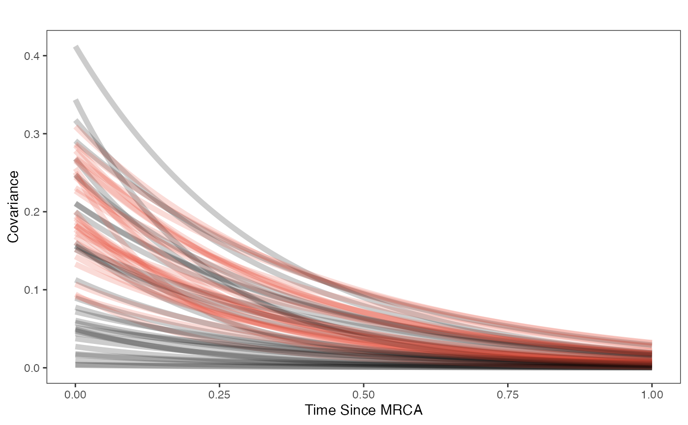

Regression Plots

########################################################################################################
#For Fig. 3
X<-dat$X_obs
Y<-dat$Y_obs

mypal <- ggsci::pal_aaas("default", alpha = 1)(3)

optima.sims<-rnorm(100,optima.prior[1],optima.prior[2])
beta.sims<-rnorm(n=100,beta.prior[1],beta.prior[2])

optima.post<-post$optima
beta.post<-data.frame(post$beta)
names(beta.post)<-c("post.beta.1","post.beta.2","post.beta.3")


mu.link.11<-function(x.seq){optima.post[,1]+x.seq*beta.post[,1]}
mu.link.12<-function(x.seq){optima.post[,2]+x.seq*beta.post[,2]}
mu.link.13<-function(x.seq){optima.post[,3]+x.seq*beta.post[,3]}


x.seq <- seq(from=min(X), to=max(X) , length.out=100)
mu.11 <- sapply(x.seq , mu.link.11 )
mu.12 <- sapply(x.seq , mu.link.12 )
mu.13 <- sapply(x.seq , mu.link.13 )


mu.mean.11<-colMeans(mu.11)
mu.mean.12<-colMeans(mu.12)
mu.mean.13<-colMeans(mu.13)


mu.mean.11<-data.frame(as.numeric(mu.mean.11))
mu.mean.12<-data.frame(as.numeric(mu.mean.12))
mu.mean.13<-data.frame(as.numeric(mu.mean.13))

names(mu.mean.11)<-"mu.mean.11"
names(mu.mean.12)<-"mu.mean.12"
names(mu.mean.13)<-"mu.mean.13"


mu.CI.11 <- apply( mu.11 , MARGIN=2, FUN=rethinking::PI , prob=0.89 )
mu.CI.12 <- apply( mu.12 , MARGIN=2, FUN=rethinking::PI , prob=0.89 )
mu.CI.13 <- apply( mu.13 , MARGIN=2, FUN=rethinking::PI , prob=0.89 )


mu.CI.11<-data.frame(t(data.frame(mu.CI.11)),x.seq)
mu.CI.12<-data.frame(t(data.frame(mu.CI.12)),x.seq)
mu.CI.13<-data.frame(t(data.frame(mu.CI.13)),x.seq)


names(mu.CI.11)<-c("min.5.5","max.94.5","x.seq")
names(mu.CI.12)<-c("min.5.5","max.94.5","x.seq")
names(mu.CI.13)<-c("min.5.5","max.94.5","x.seq")

#df<-data.frame(Y=stan_sim_data$Y,X=stan_sim_data$direct_cov)
df<-data.frame(Y=dat$Y_obs,X=dat$X_obs,Regimes=regimes_tip)
df11<-data.frame(x.seq,mu.mean.11)
df12<-data.frame(x.seq,mu.mean.12)
df13<-data.frame(x.seq,mu.mean.13)

#slope.prior.plot<-ggplot(data=reg.trdata$dat,aes(y=Sim1,x=X))+
regression.plot<-ggplot2::ggplot()+  
  ggplot2::geom_abline(intercept=optima.sims,slope=beta.sims,alpha=0.04)+ #Prior
  
  ggplot2::geom_ribbon(data=mu.CI.11,ggplot2::aes(x=x.seq,ymin=min.5.5,ymax=max.94.5),linetype=2,alpha=0.1)+
  ggplot2::geom_line(data=df11,ggplot2::aes(x=x.seq,y=mu.mean.11),linetype=1,linewidth=1,alpha=0.75,color=mypal[1])+
  ggplot2::geom_ribbon(data=mu.CI.12,ggplot2::aes(x=x.seq,ymin=min.5.5,ymax=max.94.5),linetype=2,alpha=0.1)+
  ggplot2::geom_line(data=df12,ggplot2::aes(x=x.seq,y=mu.mean.12),linetype=1,linewidth=1,alpha=0.75,color=mypal[2])+
  ggplot2::geom_ribbon(data=mu.CI.13,ggplot2::aes(x=x.seq,ymin=min.5.5,ymax=max.94.5),linetype=2,alpha=0.1)+
  ggplot2::geom_line(data=df13,ggplot2::aes(x=x.seq,y=mu.mean.13),linetype=1,linewidth=1,alpha=0.75,color=mypal[3])+
  ggplot2::geom_point(data=df,ggplot2::aes(y=Y,x=X,color=as.factor(Regimes)))+
  
  ggplot2::theme_bw()+
  ggplot2::theme(
    panel.grid.major = ggplot2::element_blank(),
    panel.grid.minor = ggplot2::element_blank())+
  
  ggplot2:: ylab("log Antler Volume (l)") + ggplot2::xlab("log Posterior Skull Length (cm)")+
  ggplot2::scale_color_manual(name="Breeding \nGroup Size",values=mypal,labels=c('1-2', '3-5', '>5'))

regression.plot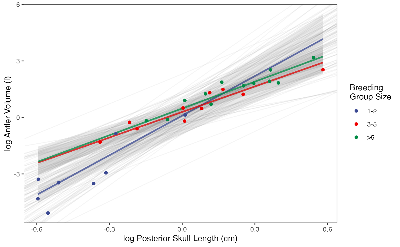


#Fig 3 in Grabowski (in press)

Let’s combine all four plots into one plot

fig2<-fig2+ggplot2::theme(legend.position="none")
fig<-ggpubr::ggarrange(hl.plot, vy.plot,covariance.plot,regression.plot,ncol=2,nrow=2, labels = c("A)","B)","C)","D)"),common.legend = TRUE,legend="top")
#ggplot2::ggsave("/Users/markgrabowski/Documents/Academic/Research/Current Projects/Blouch Project - SBR2/Blouch ms/R2/Figures/FigS9.pdf", plot = fig, width=7, height=7 )
fig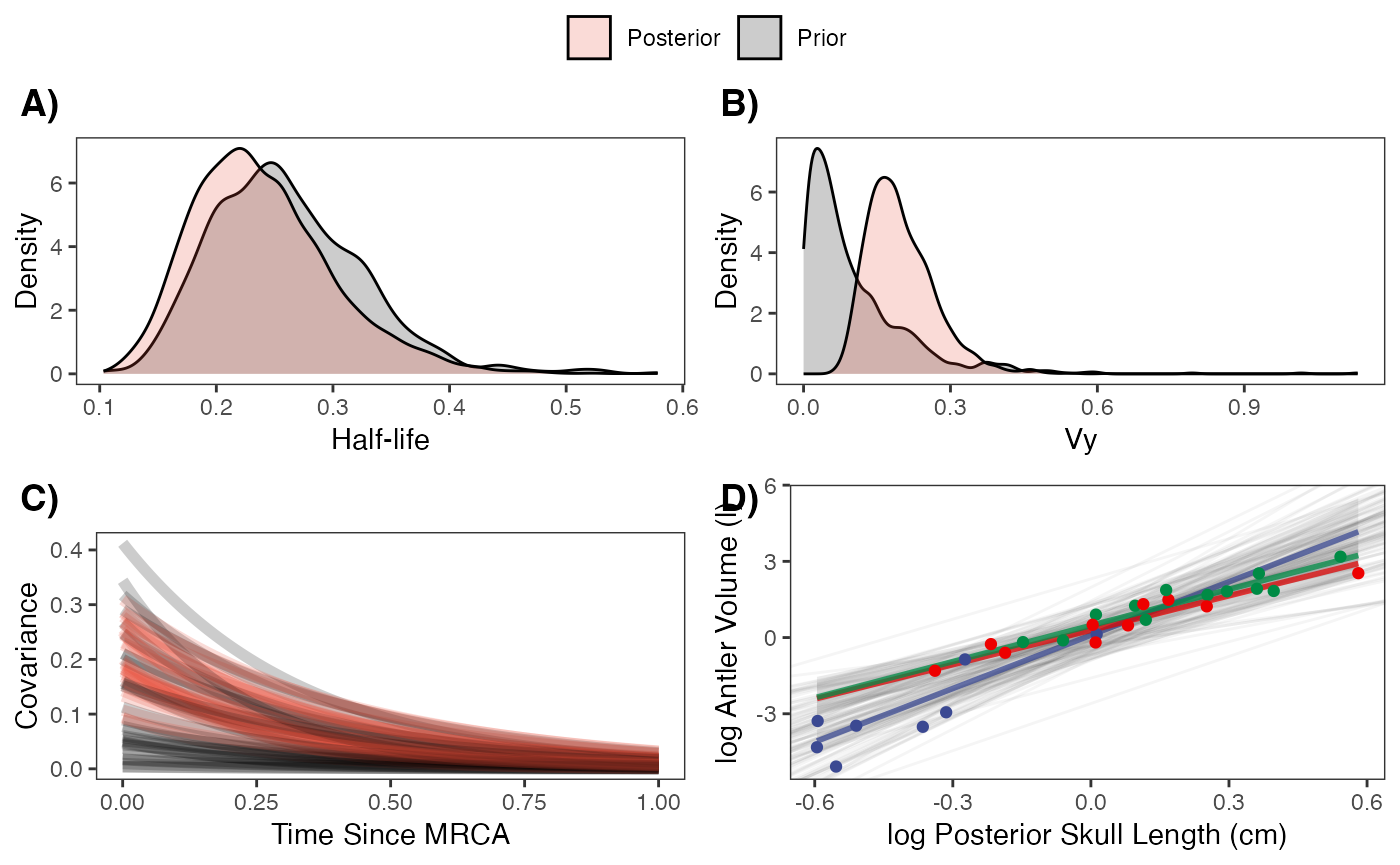

Model Comparison using PSIS

Lets do some model comparison using Pareto-Smoothed Importance Sampling (PSIS) from the R Package loo (Vehtari et al. 2023). loo estimates leave-one-out cross-validation for Bayesian analyses. Here we are looking for Pareto k values below ~0.7, which suggest the results are an accurate estimation of cross-validation. PSIS also provides a way to look at outliers in our analysis.

We then compare the two models using the loo_compare function from the same package.

dev.off()
#> null device 
#>           1
old.par <- par(mar = c(0, 0, 0, 0))
par(old.par)

############################################################################################################
loo_mlm_ve_nc <- loo::loo(fit.reg.direct.mlm.ve.nc, cores = 2, save_psis = TRUE)
#> Warning: Some Pareto k diagnostic values are too high. See help('pareto-k-diagnostic') for details.
print(loo_mlm_ve_nc)
#> 
#> Computed from 4000 by 30 log-likelihood matrix.
#> 
#>          Estimate  SE
#> elpd_loo    -26.0 4.3
#> p_loo        14.2 2.6
#> looic        51.9 8.5
#> ------
#> MCSE of elpd_loo is NA.
#> MCSE and ESS estimates assume MCMC draws (r_eff in [0.5, 1.5]).
#> 
#> Pareto k diagnostic values:
#>                          Count Pct.    Min. ESS
#> (-Inf, 0.7]   (good)     23    76.7%   214     
#>    (0.7, 1]   (bad)       7    23.3%   <NA>    
#>    (1, Inf)   (very bad)  0     0.0%   <NA>    
#> See help('pareto-k-diagnostic') for details.
plot(loo_mlm_ve_nc)
plot(loo_mlm_ve_nc,label_points=TRUE)


#library(loo) #Non-mlm varying effects model
loo_ve <- loo::loo(fit.reg.direct.ve, cores = 2, save_psis = TRUE)
#> Warning: Some Pareto k diagnostic values are too high. See help('pareto-k-diagnostic') for details.
print(loo_ve)
#> 
#> Computed from 4000 by 30 log-likelihood matrix.
#> 
#>          Estimate  SE
#> elpd_loo    -25.2 4.2
#> p_loo        13.8 2.6
#> looic        50.4 8.5
#> ------
#> MCSE of elpd_loo is NA.
#> MCSE and ESS estimates assume MCMC draws (r_eff in [0.5, 1.7]).
#> 
#> Pareto k diagnostic values:
#>                          Count Pct.    Min. ESS
#> (-Inf, 0.7]   (good)     23    76.7%   496     
#>    (0.7, 1]   (bad)       6    20.0%   <NA>    
#>    (1, Inf)   (very bad)  1     3.3%   <NA>    
#> See help('pareto-k-diagnostic') for details.
plot(loo_ve)
plot(loo_ve,label_points=TRUE)


#library(loo) #MLM Varying intercepts model
loo_mlm_vi_nc <- loo::loo(fit.reg.direct.mlm.vi.nc, cores = 2, save_psis = TRUE)
#> Warning: Some Pareto k diagnostic values are too high. See help('pareto-k-diagnostic') for details.
print(loo_mlm_vi_nc)
#> 
#> Computed from 4000 by 30 log-likelihood matrix.
#> 
#>          Estimate   SE
#> elpd_loo    -28.3  5.3
#> p_loo        12.9  3.3
#> looic        56.7 10.6
#> ------
#> MCSE of elpd_loo is NA.
#> MCSE and ESS estimates assume MCMC draws (r_eff in [0.4, 1.2]).
#> 
#> Pareto k diagnostic values:
#>                          Count Pct.    Min. ESS
#> (-Inf, 0.7]   (good)     24    80.0%   152     
#>    (0.7, 1]   (bad)       6    20.0%   <NA>    
#>    (1, Inf)   (very bad)  0     0.0%   <NA>    
#> See help('pareto-k-diagnostic') for details.
plot(loo_mlm_vi_nc)
plot(loo_mlm_vi_nc,label_points=TRUE)


#library(loo) #Basic model
loo_basic <- loo::loo(fit.reg.direct, cores = 2, save_psis = TRUE)
#> Warning: Some Pareto k diagnostic values are too high. See help('pareto-k-diagnostic') for details.
print(loo_basic)
#> 
#> Computed from 4000 by 30 log-likelihood matrix.
#> 
#>          Estimate   SE
#> elpd_loo    -27.8  5.1
#> p_loo        12.3  3.1
#> looic        55.6 10.3
#> ------
#> MCSE of elpd_loo is NA.
#> MCSE and ESS estimates assume MCMC draws (r_eff in [0.5, 1.9]).
#> 
#> Pareto k diagnostic values:
#>                          Count Pct.    Min. ESS
#> (-Inf, 0.7]   (good)     26    86.7%   416     
#>    (0.7, 1]   (bad)       4    13.3%   <NA>    
#>    (1, Inf)   (very bad)  0     0.0%   <NA>    
#> See help('pareto-k-diagnostic') for details.
plot(loo_basic)
plot(loo_basic,label_points=TRUE)

loo::loo_compare(loo_mlm_ve_nc, loo_ve, loo_mlm_vi_nc, loo_basic)
#>        elpd_diff se_diff
#> model2  0.0       0.0   
#> model1 -0.7       0.9   
#> model4 -2.6       3.6   
#> model3 -3.1       3.6
2.6 + c(-1,1)*3.3*1.86 #95% interval of the difference, z-score of 1.86
#> [1] -3.538  8.738

Model Comparison using Bayes Factors

Now lets compare our two models using Bayes Factors. Here we use the bridgesampling R package (Gronau et al. 2020). Looking below, we can read the results as the data is X times more likely under a model that assumes the first mode rather than second model.

############################################################################################################
lml.fit.reg.direct.mlm.ve.nc<-bridgesampling::bridge_sampler(fit.reg.direct.mlm.ve.nc,silent=TRUE)
lml.fit.reg.direct.mlm.vi.nc<-bridgesampling::bridge_sampler(fit.reg.direct.mlm.vi.nc,silent=TRUE)
lml.fit.reg.direct.ve<-bridgesampling::bridge_sampler(fit.reg.direct.ve,silent=TRUE)
lml.fit.reg.direct<-bridgesampling::bridge_sampler(fit.reg.direct,silent=TRUE)

#bridgesampling::bf(lml.fit.reg.direct.mlm.ve, lml.fit.reg.direct.mlm.ve.nc)
bridgesampling::bf(lml.fit.reg.direct.ve, lml.fit.reg.direct.mlm.ve.nc)
#> Estimated Bayes factor in favor of lml.fit.reg.direct.ve over lml.fit.reg.direct.mlm.ve.nc: 13.81466
bridgesampling::bf(lml.fit.reg.direct.ve, lml.fit.reg.direct.mlm.vi.nc)
#> Estimated Bayes factor in favor of lml.fit.reg.direct.ve over lml.fit.reg.direct.mlm.vi.nc: 59.28168
bridgesampling::bf(lml.fit.reg.direct.ve, lml.fit.reg.direct)
#> Estimated Bayes factor in favor of lml.fit.reg.direct.ve over lml.fit.reg.direct: 9.73733

Trace for estimated parameters

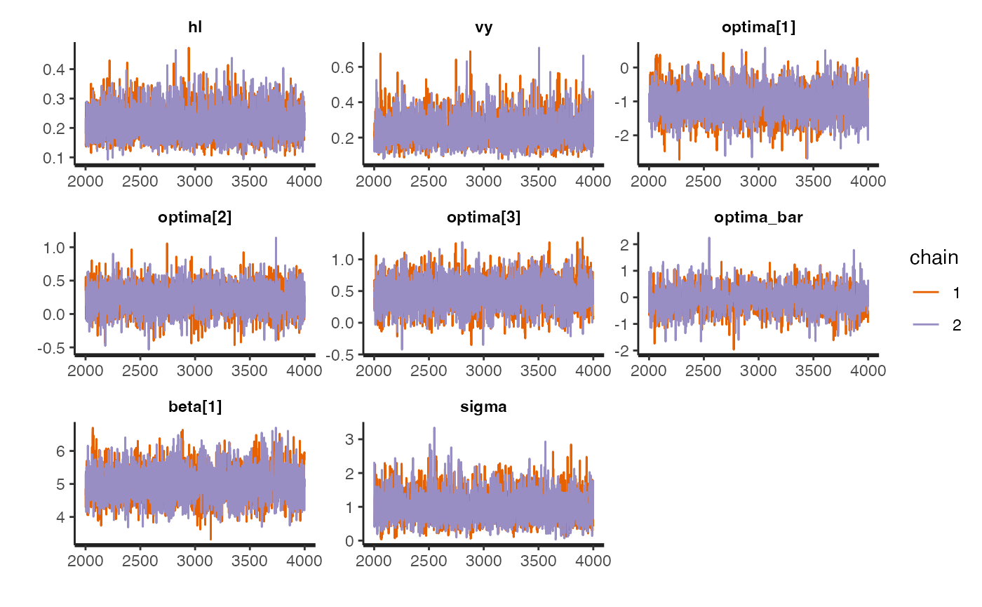
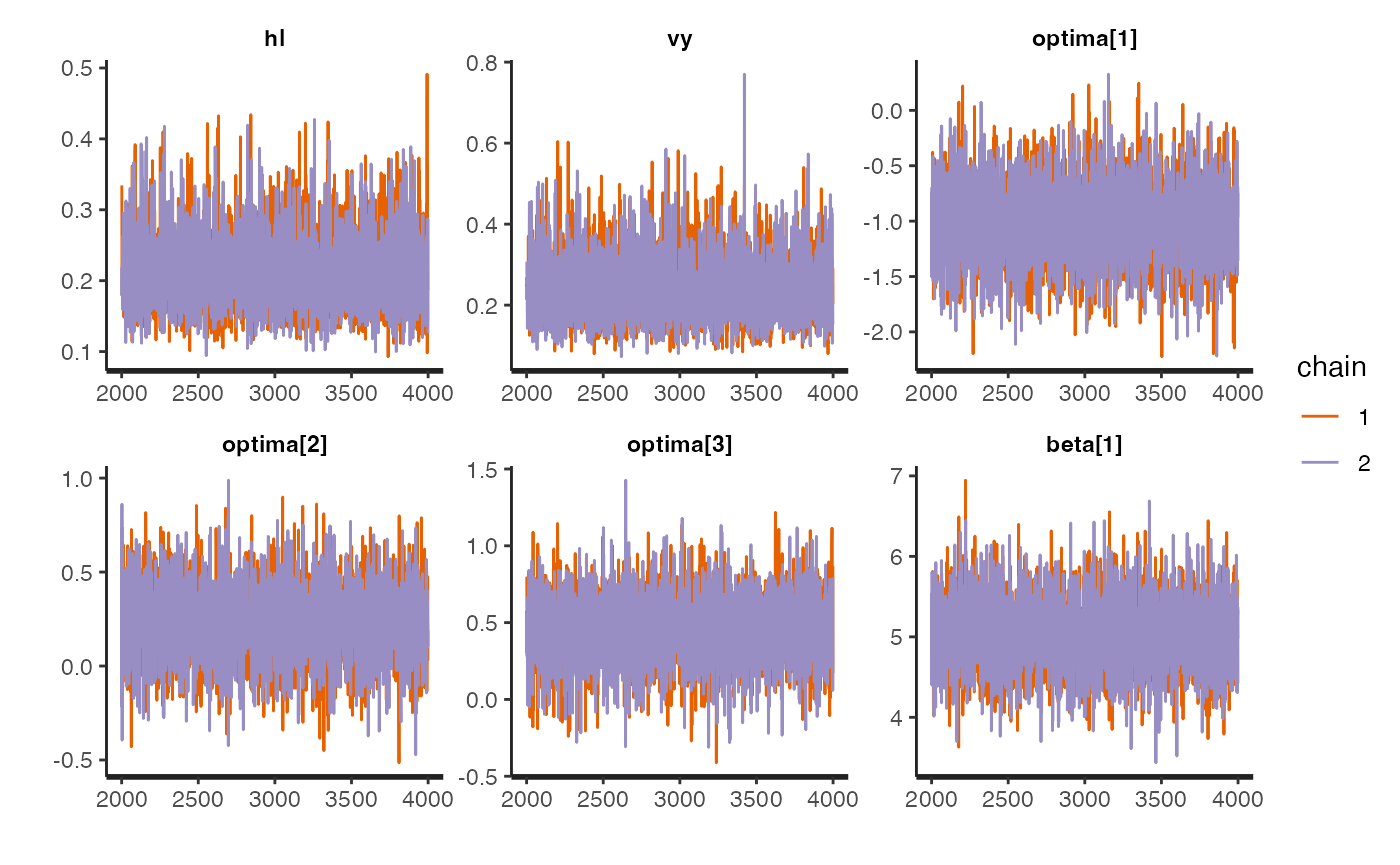
Let’s look at traceplots of our models, which give a visualization of degree of convergence.

############################################################################################################
#Trankplots/Traceplots 4X10
rstan::traceplot(fit.reg.direct.ve,pars = c("hl","vy","optima","beta"))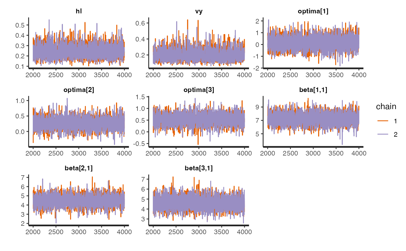

rstan::traceplot(fit.reg.direct.mlm.ve.nc,pars = c("hl","vy","optima_bar","beta_bar","Rho","sigma","optima","beta"))

rstan::traceplot(fit.reg.direct.mlm.vi.nc,pars = c("hl","vy","optima","optima_bar","beta","sigma"))

rstan::traceplot(fit.reg.direct,pars = c("hl","vy","optima","beta"))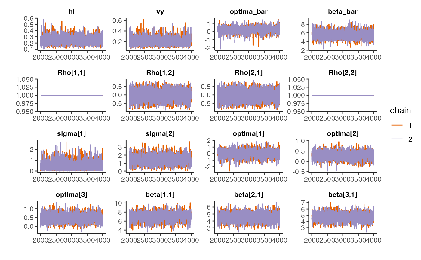


#plot.emp.ve<-rstan::traceplot(fit.reg.direct.ve,pars = c("hl","vy","optima","beta"))
#plot.emp.mlm.ve<-rstan::traceplot(fit.reg.direct.mlm.ve.nc,pars = c("hl","vy","optima_bar","beta_bar","Rho","sigma","optima","beta"))
#plot.emp.vi<-rstan::traceplot(fit.reg.direct.ve,pars = c("hl","vy","optima","beta"))
#plot.emp.mlm.vi<-rstan::traceplot(fit.reg.direct.mlm.ve.nc,pars = c("hl","vy","optima","optima_bar","beta","sigma"))

#fig<-ggpubr::ggarrange(plot.emp.vi, plot.emp.ve,plot.emp.mlm.vi,plot.emp.mlm.ve,ncol=2,nrow=2, labels = c("A)","B)","C)","D)"),common.legend = TRUE,legend="top")
#fig<-ggpubr::annotate_figure(fig,top=paste("Multi-Optima Direct Effect - Varying Effects, hl=",hl,sep=""))
#ggplot2::ggsave("/Users/markgrabowski/Documents/Academic/Research/Current Projects/Blouch Project - SBR2/Blouch ms/R2/Figures/FigS6.pdf", plot = fig, width=9, height=9)
########################################################################################################

Compare posterior distributions

Now that we have our best model, lets compare the posterior distributions of slopes and other usuful stats

########################################################################################################
#Compare slopes
df<-data.frame(post.ve$beta)
mean(df[,1]-df[,2])
#> [1] 2.800276
rethinking::PI(df[,1]-df[,2],prob=0.95)
#>        3%       98% 
#> 0.7948055 4.8046596
sum((df[,1]-df[,2])<0)/4000
#> [1] 0.00275
sum((df[,1]-df[,2])>=0)/4000
#> [1] 0.99725

unscaled.hl<-post.ve$hl*l.tree
mean(unscaled.hl)
#> [1] 3.384105
rethinking::PI(unscaled.hl,prob=0.95)
#>       3%      98% 
#> 2.030006 5.282994

Predictive Checks

Now lets run prior and posterior predictive checks for our two models. Prior predictive checks generate predictions from the model using only the prior distributions in order to assess whether the priors are appropriate – they are equivalent to running the model without data (Gabry et al. 2019). Posterior predictive checks generate data according to the posterior predictive distribution and compare it to the observed data to assess the fit of the model (Gabry et al. 2019). Blouch includes Stan functions to run prior and posterior predictive checks for each of the included models and their use is demonstrated below in the simulation and empirical examples.

dat<-blouch.reg.direct.prep(trdata,"Y_with_error","Y_error","X_with_error","X_error",Z_direct=1,"BGS",hl.prior,vy.prior,optima.prior,beta.prior)

fit.reg.direct.ve.priorpc<- rstan::sampling(object = blouch:::stanmodels$blouchOU_reg_direct_ve_priorpc,data=dat,chains = 2,cores=2, iter =2000,algorithm=c("Fixed_param"))
#> Found more than one class "stanfit" in cache; using the first, from namespace 'rstan'
#> Also defined by 'rethinking'
#> Found more than one class "stanfit" in cache; using the first, from namespace 'rstan'
#> Also defined by 'rethinking'

post<-rstan::extract(fit.reg.direct.ve.priorpc)

num.plots<-5
plots<-ysim.ppc.plot.code(dat,post,1:num.plots)
plots<-gridExtra::grid.arrange(grobs=plots, ncol=5, nrow=1,common.legend=TRUE,legend="top")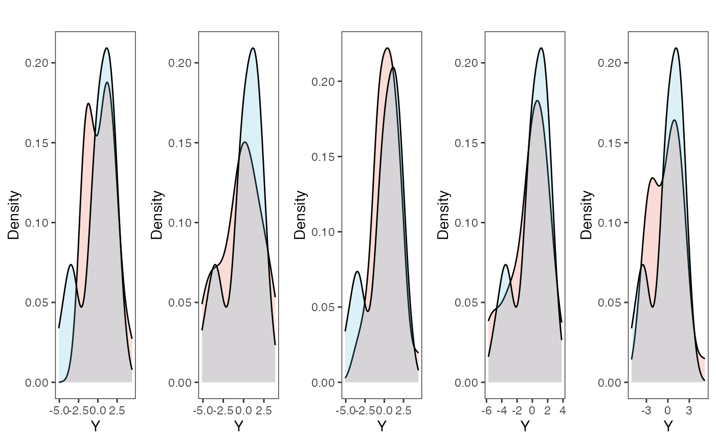

tgrob <- ggpubr::text_grob("Multi-Optima Direct Effect Model - Varying Efects - Prior PC",size = 10)
plots.prior<-ggpubr::annotate_figure(plots,top=tgrob)

fit.reg.direct.ve.postpc<- rstan::sampling(object = blouch:::stanmodels$blouchOU_reg_direct_ve_postpc,data=dat,chains = 2,cores=2, iter =2000)
#> Found more than one class "stanfit" in cache; using the first, from namespace 'rstan'
#> Also defined by 'rethinking'
#> Found more than one class "stanfit" in cache; using the first, from namespace 'rstan'
#> Also defined by 'rethinking'


post<-rstan::extract(fit.reg.direct.ve.postpc)

num.plots<-5
plots<-ysim.ppc.plot.code(dat,post,1:num.plots)
plots<-gridExtra::grid.arrange(grobs=plots, ncol=5, nrow=1,common.legend=TRUE,legend="top")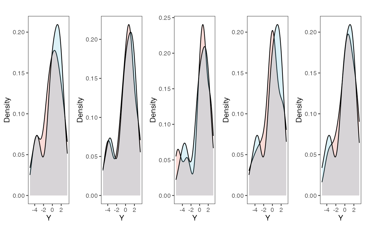

tgrob <- ggpubr::text_grob("Multi-Optima Direct Effect Model - Varying Efects - Posterior PC",size = 10)
plots.post<-ggpubr::annotate_figure(plots,top=tgrob)
fig<-ggpubr::ggarrange(plots.prior, plots.post,ncol=1,nrow=2, labels = c("C)","D)"),common.legend = TRUE,legend="top")

plots.prior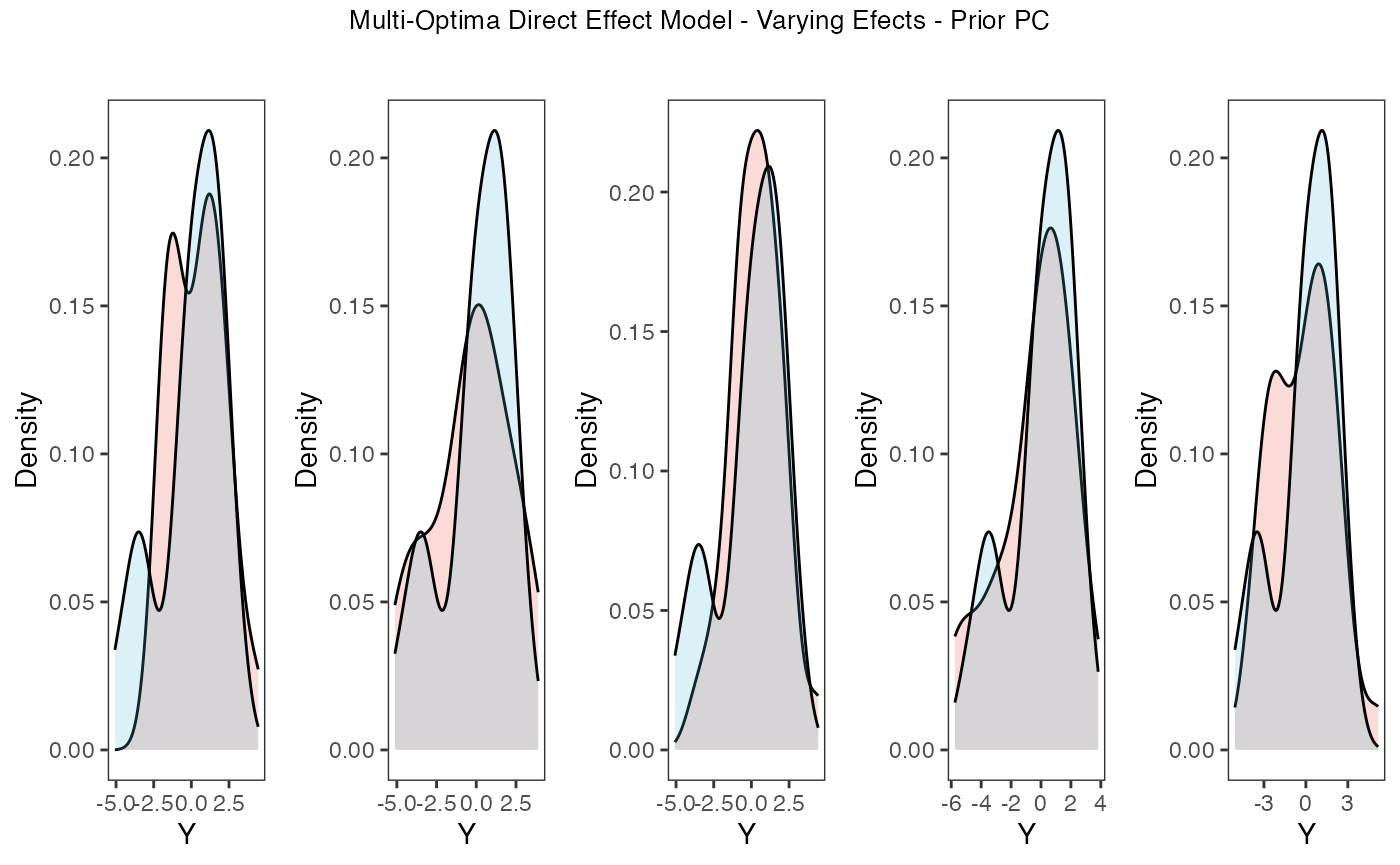

plots.post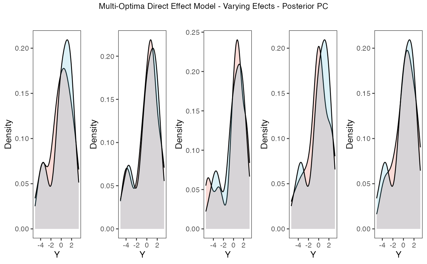

Posterior predictive checks show that the model is well fit as it generates data that are a close approximation of the true dataset.

References

Pagel, M (1994) Detecting correlated evolution on phylogenies: a general method for the comparative analysis of discrete characters. Proceedings of the Royal Society of London. Series B. Biological Sciences, 255, 37–445.

Tsuboi M., Kopperud B.T., Matschiner M., Grabowski M., Syrowatka C., Pélabon C., Hansen T.F. 2024. Antler Allometry, the Irish Elk and Gould Revisited. Evol Biol.

Mark Grabowski

2024-10-08

Background

Load datasets

Combine data and tree and paint regimes on tree.

Setup dataset and add measurement errors

Setting Priors

Exploring Priors

Explore Priors - built in functions

Data setup for Blouch

Running models

Priors vs. posterior plots for multi-optima direct effect model

Multi-optima direct effect model with varying effects

Priors vs. posterior plots for multi-optima direct effect model with varying effects

Multilevel Models

Multilevel Multi-Optima Direct Effect Model with Varying Intercepts

Priors vs. posterior plots for multilevel multi-optima direct effect model with varying intercepts

Multilevel Multi-Optima Direct Effect Model with Varying Effects

Priors vs. posterior plots for multilevel multi-optima direct effect model with varying effects

Model Comparison using PSIS

Model Comparison using Bayes Factors

Trace for estimated parameters

Compare posterior distributions

Predictive Checks

References