Mullti-Optima Models Walkthrough

Mark Grabowski

2024-10-08

rm(list=ls())

library(blouch)

########################################################################################################
#For execution on a local, multicore CPU with excess RAM we recommend calling
#options(mc.cores = parallel::detectCores())
options(mc.cores = 2) #2 For R package checks - use line above on your own machine
rstan::rstan_options(auto_write = TRUE)

dotR <- file.path(Sys.getenv("HOME"), ".R")
if (!file.exists(dotR)) dir.create(dotR)
M <- file.path(dotR, "Makevars")
if (!file.exists(M)) file.create(M)
arch <- ifelse(R.version$arch == "aarch64", "arm64", "x86_64")
cat(paste("\nCXX14FLAGS += -O3 -mtune=native -arch", arch, "-ftemplate-depth-256"),
    file = M, sep = "\n", append = FALSE)

Multi-optima Model

Next we will run a series of models that include categorical variables - regimes painted on a phylogeny following Hansen (1997) and Hansen et al. (2008). This article is an abbreviated versions of the Simulation Example article - most of the steps of analysis will be the same and are not repeated here. Note that the Stan runs are also too few iterations and use only 1 chain and 1 core.

First we will set up the regime painting

########################################################################################################
#Create phylogeny
########################################################################################################
N<-50 #Number of species
set.seed(10) #Set seed to get same random species each time

phy <- ape::keep.tip(tree.10K,sample(tree.10K$tip.label)[1:N]) 
phy<-ape::multi2di(phy)

l.tree<-max(ape::branching.times(phy)) ## rescale tree to height 1
phy$edge.length<-phy$edge.length/l.tree 

tip.label<-phy$tip.label


#Set regimes - manually - 2 regimes
#Locate nodes
plot(phy,no.margin=TRUE,edge.width=2,cex=0.7)
ape::nodelabels(frame="none",adj=c(1.1,-0.4))
ape::tiplabels()

#Paint Regimes on Tree
#source("/Users/markgrabowski/Documents/Academic/Research/Current Projects/Blouch project/blouch/Simulation Code/Functions/set.converge.regimes.R") #Macbook Pro

shifts<-c(84) #Location of nodes with regime shifts
trdata<-data.frame(phy$tip.label)
trdata<-treeplyr::make.treedata(phy,trdata)
trdata<-set.converge.regimes(trdata,shifts)
#> [1] 1
#>  [1] OU1 OU1 OU1 OU1 OU1 OU1 OU1 OU1 OU1 OU1 OU1 OU1 OU1 OU1 OU1 OU1 OU1 OU1 OU1
#> [20] OU1 OU1 OU1 OU1 OU1 OU1 OU1 OU1 OU1 OU1 OU1 OU1 OU1 OU1 OU1 OU1 OU1 OU1 OU1
#> [39] OU1 OU1 OU1 OU1 OU1 OU1 OU1 OU1 OU1 OU1 OU1 OU1 OU1 OU1 OU1 OU1 OU1 OU1 OU1
#> [58] OU1 OU1 OU1 OU1 OU1 OU1 OU1 OU2 OU2 OU2 OU2 OU2 OU2 OU2 OU2 OU2 OU2 OU2 OU2
#> [77] OU2 OU2 OU2 OU2 OU2 OU2 OU2 OU2 OU2 OU1 OU1 OU1 OU1 OU1 OU1 OU1 OU1 OU1 OU1
#> [96] OU1 OU1 OU1
#> Levels: OU1 OU2
#> [1] "#E64B35FF" "#4DBBD5FF"

#Check if manual setting code worked
shifts.total<-c(trdata$dat$regimes,trdata$phy$node.label)
edge.regimes <- factor(shifts.total[trdata$phy$edge[,2]])
print(edge.regimes)
#>  [1] OU1 OU1 OU1 OU1 OU1 OU1 OU1 OU1 OU1 OU1 OU1 OU1 OU1 OU1 OU1 OU1 OU1 OU1 OU1
#> [20] OU1 OU1 OU1 OU1 OU1 OU1 OU1 OU1 OU1 OU1 OU1 OU1 OU1 OU1 OU1 OU1 OU1 OU1 OU1
#> [39] OU1 OU1 OU1 OU1 OU1 OU1 OU1 OU1 OU1 OU1 OU1 OU1 OU1 OU1 OU1 OU1 OU1 OU1 OU1
#> [58] OU1 OU1 OU1 OU1 OU1 OU1 OU1 OU2 OU2 OU2 OU2 OU2 OU2 OU2 OU2 OU2 OU2 OU2 OU2
#> [77] OU2 OU2 OU2 OU2 OU2 OU2 OU2 OU2 OU2 OU1 OU1 OU1 OU1 OU1 OU1 OU1 OU1 OU1 OU1
#> [96] OU1 OU1 OU1
#> Levels: OU1 OU2

reg.colors <- ggsci::pal_aaas("default", alpha = 0.7)(2)
print(reg.colors)
#> [1] "#3B4992B2" "#EE0000B2"
plot(trdata$phy,edge.color = reg.colors[edge.regimes], edge.width = 1, cex = 0.2)

Format tree

############################################################################################################
#Simulate data
n<-length(trdata$phy$tip.label)
regimes_internal <-trdata$phy$node.label
regimes_tip <- trdata$dat$regimes
regimes <- concat.factor(regimes_tip, regimes_internal)
anc_maps<-"regimes"
lineages <- lapply(1:n, function(e) lineage.constructor(trdata$phy, e, anc_maps, regimes)) #Trace lineage from tips (n) to root and determine regimes of each node or branch

Now we will simulate Y data based on our generative model

############################################################################################################
#Set true values for parameters
hl<-0.1 #0.1, 0.25, 0.75 - testing options
a<-log(2)/hl
vy<-0.01 #0.25,0.5 - testing options
sigma2_y<-vy*(2*(log(2)/hl));
optima<-c(0.5,0.25) #Optima for two regimes

dmX<-weight.matrix(trdata$phy, a, lineages) #Slouch approach
mu<-dmX%*%optima #Simulate mu for Y
V<-calc_direct_V(phy, sigma2_y, a)
Y<-MASS::mvrnorm(n=1,mu,V)

########################################################################################################
#Simulate errors
Y_error<-rep(0.01,N)
Y_with_error<-Y+rnorm(N,0,0.01)

phytools::phenogram(phy,Y_with_error,spread.labels=TRUE,spread.cost=c(1,0)) #Plot X data
#> Optimizing the positions of the tip labels...

############################################################################################################
#Make trdata file
trait.data<-data.frame(cbind(Y_with_error,Y_error))
trdata$dat<-cbind(trdata$dat,data.frame(cbind(Y_with_error,Y_error)))

############################################################################################################

############################################################################################################
#Set Priors
hl.prior<-c(log(0.25),0.75)
vy.prior<-20
optima.prior<-c(0,1) #Informed by linear model

Exploring Priors

At this point one would want to explore if the priors are appropriate - do the prior distributions look consistent with what we know about our system? See Grabowski (in press) for more on setting priors.

Half-life Prior plot

hl.sims<-data.frame(rlnorm(n=1000,meanlog=hl.prior[1],sdlog=hl.prior[2]))
names(hl.sims)<-"prior.hl.sims"

hl.prior.plot<-ggplot2::ggplot()+
  ggplot2::geom_density(ggplot2::aes(prior.hl.sims,fill="prior.hl.sims"),alpha=0.2,data=hl.sims)+
  ggplot2::theme_bw()+
  ggplot2::theme(
    panel.grid.major = ggplot2::element_blank(),
    panel.grid.minor = ggplot2::element_blank())+
  
  #labs(title="Prior vs. Posterior Distribution ",x="Half-life", y = "Density")+
  ggplot2::labs(title="",x="Half-life", y = "Density")+
  
  #scale_fill_manual(labels=c("Posterior","Prior"))+
  ggplot2::geom_vline(xintercept=c(hl),linetype=2)+
  ggsci::scale_fill_npg(name="",labels=c("Prior"))

hl.prior.plot

Vy Prior Plot

vy.sims<-rexp(n=1000,rate=vy.prior)
vy.sims<-data.frame(vy.sims)
names(vy.sims)<-"prior.vy.sims"

vy.prior.plot<-ggplot2::ggplot()+
  ggplot2::geom_density(ggplot2::aes(prior.vy.sims,fill="prior.vy.sims"),alpha=0.2,data=vy.sims)+
  ggplot2::theme_bw()+
  ggplot2::theme(
    panel.grid.major = ggplot2::element_blank(),
    panel.grid.minor = ggplot2::element_blank())+
  
  #labs(title="Prior vs. Posterior Distribution ",x="vy", y = "Density")+
  ggplot2::labs(title="",x="vy", y = "Density")+
  ggplot2::geom_vline(xintercept=c(vy),linetype=2)+
  
  #scale_fill_manual(labels=c("Posterior","Prior"))+
  ggsci::scale_fill_npg(name="",labels=c("Prior"))


vy.prior.plot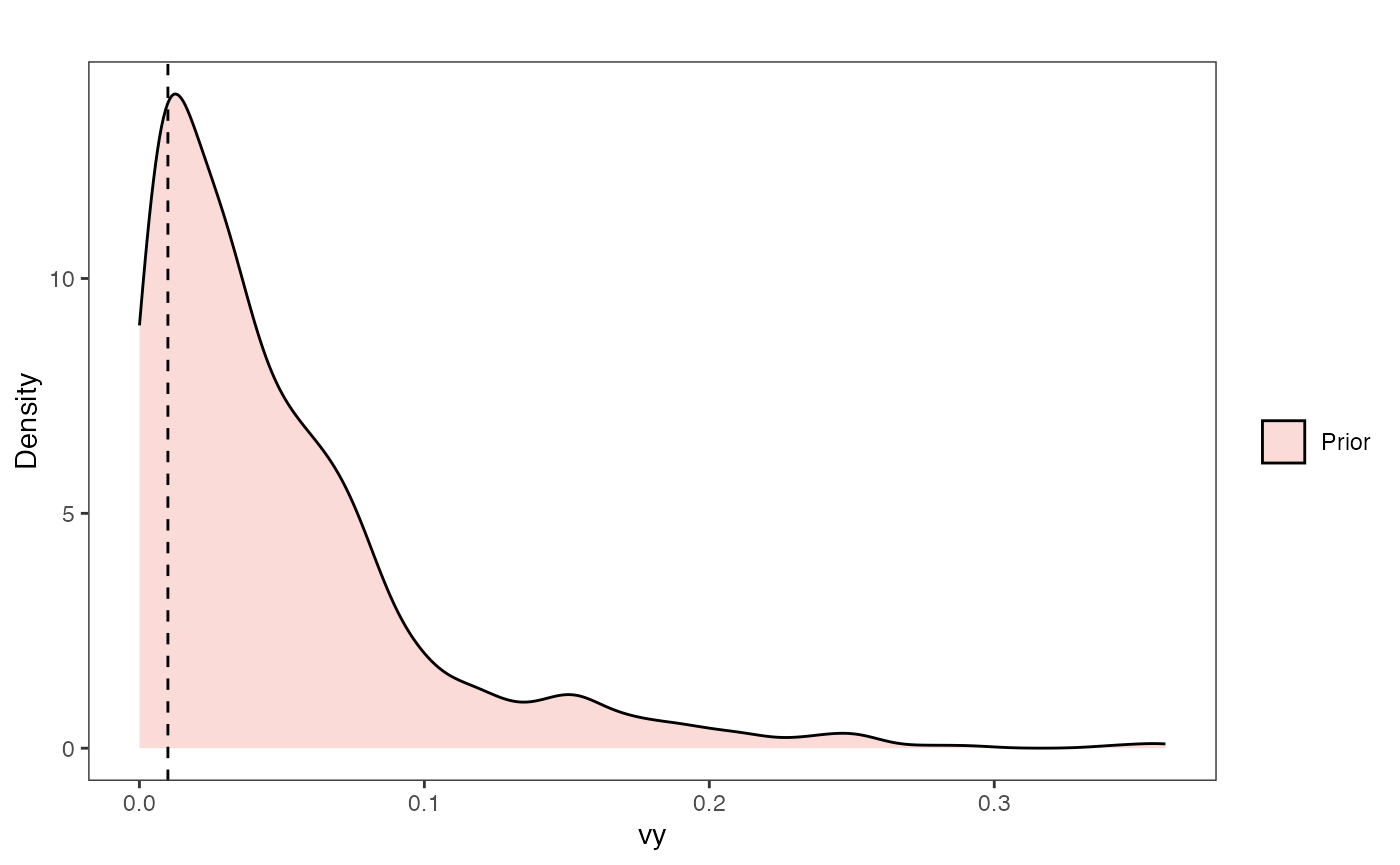

Prior on how shared branch lengths correspond to covariance

a.sims<-log(2)/hl.sims;
sigma2_y.sims<-vy.sims*(2*(log(2)/hl.sims));
#x<-seq(from=0,to=1,by=0.001)
#V.sim<-calc_direct_V(phy,a.sims,sigma2_y.sims)

plot( NULL , xlim=c(0,1) , ylim=c(0,0.3) , xlab="Time since MRCA" , ylab="Covariance" ,cex.axis=0.75, mgp=c(1.25,0.25,0),tcl=-0.25)
for (i in 1:30){
  curve(sigma2_y.sims[i,] /(2 * a.sims[i,]) * ((1 - exp(-2 * a.sims[i,] * (1-(x/2)))) * exp(-a.sims[i,] * x)) , add=TRUE , lwd=4 , col=rethinking::col.alpha(1,0.15))
}

par(mar=c(3,3,0.25,0.25))
covariance.prior.plot <- recordPlot()
dev.off()
#> null device 
#>           1
covariance.prior.plot

Prior Plot

library(ggsci)

#Direct Model
#intercept_test<-rnorm(100,stan_sim_data$ols_intercept,0.2)
#slope_test<-rnorm(100,stan_sim_data$ols_slope,0.1)

optima.sims<-rnorm(100,optima.prior[1],optima.prior[2])
optima.sims<-data.frame(optima.sims,Prior="Prior")

df<-data.frame(Y=Y,regimes=regimes_tip)
names(df)<-c("Y","Regimes")

optima.plot<-
  ggplot2::ggplot(data=df, Mapping = ggplot2::aes(x = Y, y = Regimes))+
  
  ggplot2::geom_jitter(data=optima.sims,ggplot2::aes(y=optima.sims,x=Prior),alpha=0.25,width=0.15)+
  ggplot2::geom_jitter(data=df,ggplot2::aes(y=Y,x=Regimes),width=0.15)+
  ggplot2::theme_bw()+
  ggplot2::ylab("Optima") + ggplot2::xlab("")+
  ggsci::scale_color_npg()

optima.plot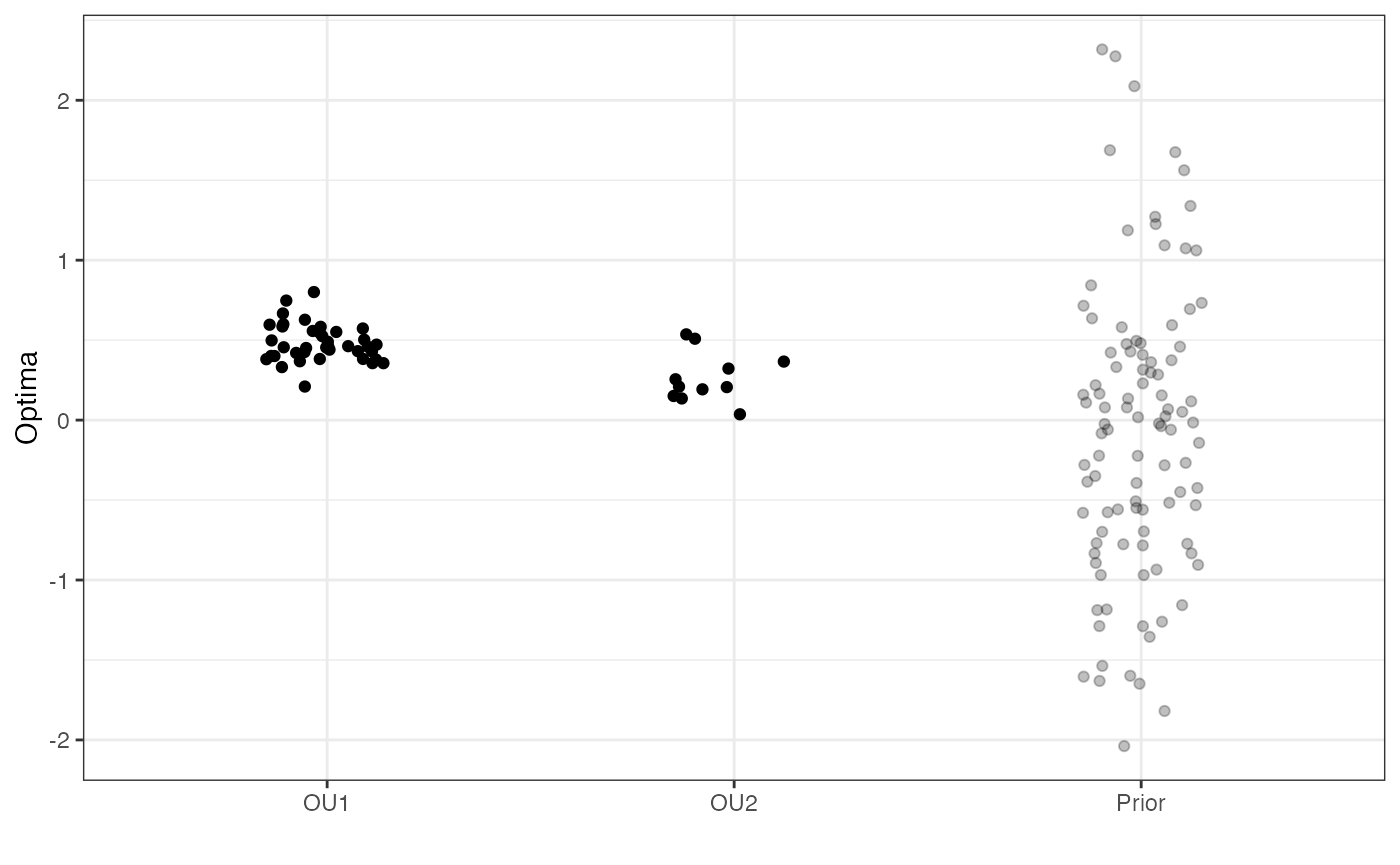

We will use the helper function blouch.reg.prep() to setup the dat file for Stan. Here “regimes” is the name of the regime column in trdata$dat.

dat<-blouch.reg.prep(trdata,"Y_with_error","Y_error","regimes",hl.prior,vy.prior,optima.prior)

Here we run the basic Multi-optima Model, look at the results, and rstan::extract the posterior

fit.reg<- rstan::sampling(object = blouch:::stanmodels$blouchOU_reg,data = dat,chains = 2,iter =2000,cores=2)
#> Found more than one class "stanfit" in cache; using the first, from namespace 'rstan'
#> Also defined by 'rethinking'
#> Found more than one class "stanfit" in cache; using the first, from namespace 'rstan'
#> Also defined by 'rethinking'

print(fit.reg,pars = c("hl","vy","optima"))
#> Inference for Stan model: blouchOU_reg.
#> 2 chains, each with iter=2000; warmup=1000; thin=1; 
#> post-warmup draws per chain=1000, total post-warmup draws=2000.
#> 
#>           mean se_mean   sd 2.5%  25%  50%  75% 97.5% n_eff Rhat
#> hl        0.09       0 0.05 0.03 0.06 0.09 0.11  0.21  1072    1
#> vy        0.02       0 0.01 0.01 0.02 0.02 0.02  0.03  1055    1
#> optima[1] 0.47       0 0.03 0.40 0.46 0.48 0.50  0.54  1892    1
#> optima[2] 0.27       0 0.05 0.15 0.23 0.27 0.30  0.37  1766    1
#> 
#> Samples were drawn using NUTS(diag_e) at Tue Oct  8 13:46:11 2024.
#> For each parameter, n_eff is a crude measure of effective sample size,
#> and Rhat is the potential scale reduction factor on split chains (at 
#> convergence, Rhat=1).
post<-rstan::extract(fit.reg) #rstan::extract posterior

Now lets look at the prior vs. posterior plots for the parameters Half-life plot

hl.post<-data.frame(post$hl)
names(hl.post)<-"post.hl.sims"

hl.plot<-ggplot2::ggplot()+
  ggplot2::geom_density(ggplot2::aes(prior.hl.sims,fill="prior.hl.sims"),alpha=0.2,data=hl.sims)+
  ggplot2::geom_density(ggplot2::aes(post.hl.sims,fill="post.hl.sims"),alpha=0.2,data=hl.post)+
  ggplot2::theme_bw()+
  ggplot2::theme(
    panel.grid.major = ggplot2::element_blank(),
    panel.grid.minor = ggplot2::element_blank())+
  
  #labs(title="Prior vs. Posterior Distribution ",x="Half-life", y = "Density")+
  ggplot2::labs(title="",x="Half-life", y = "Density")+
  
  #scale_fill_manual(labels=c("Posterior","Prior"))+
  ggplot2::geom_vline(xintercept=c(hl),linetype=2)+
  ggsci::scale_fill_npg(name="",labels=c("Posterior","Prior"))

hl.plot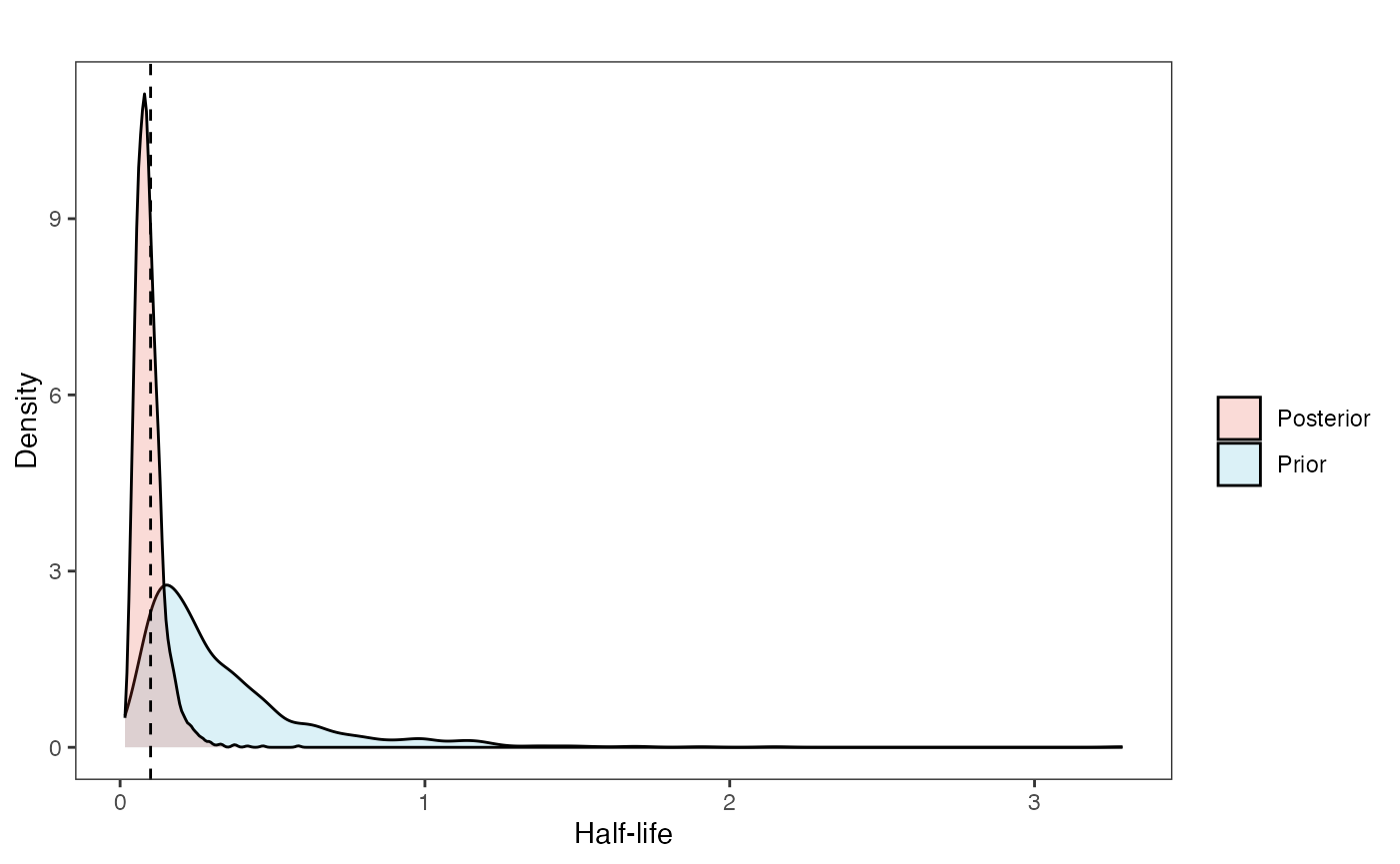

Vy Prior vs. posterior plot

vy.post<-data.frame(post$vy)
names(vy.post)<-"post.vy.sims"


vy.plot<-ggplot2::ggplot()+
  ggplot2::geom_density(ggplot2::aes(prior.vy.sims,fill="prior.vy.sims"),alpha=0.2,data=vy.sims)+
  ggplot2::geom_density(ggplot2::aes(post.vy.sims,fill="post.vy.sims"),alpha=0.2,data=vy.post)+
  ggplot2::theme_bw()+
  ggplot2::theme(
    panel.grid.major = ggplot2::element_blank(),
    panel.grid.minor = ggplot2::element_blank())+
  
  #labs(title="Prior vs. Posterior Distribution ",x="vy", y = "Density")+
  ggplot2::labs(title="",x="vy", y = "Density")+
  ggplot2::geom_vline(xintercept=c(vy),linetype=2)+
  
  #scale_fill_manual(labels=c("Posterior","Prior"))+
  ggsci::scale_fill_npg(name="",labels=c("Posterior","Prior"))

vy.plot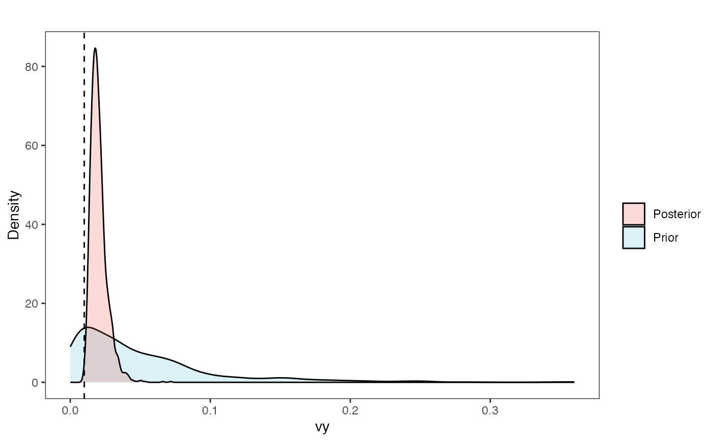

Prior versus posterior on how shared branch lengths correspond to covariance

plot( NULL , xlim=c(0,1) , ylim=c(0,0.3) , xlab="Time since MRCA" , ylab="Covariance" ,cex.axis=0.75, mgp=c(1.25,0.25,0),tcl=-0.25)
for (i in 1:30){
  curve(sigma2_y.sims[i,] /(2 * a.sims[i,]) * ((1 - exp(-2 * a.sims[i,] * (1-(x/2)))) * exp(-a.sims[i,] * x)) , add=TRUE , lwd=4 , col=rethinking::col.alpha(1,0.15))
}

for (i in 1:30){
  curve(post$sigma2_y[i] /(2 * post$a[i]) * ((1 - exp(-2 * post$a[i] * (1-(x/2)))) * exp(-post$a[i] * x)) , add=TRUE , lwd=4 , col=rethinking::col.alpha(2,0.5))
}

par(mar=c(3,3,0.25,0.25))
#covariance.plot <- recordPlot()
#dev.off()

Prior vs. Posterior Plot

library(ggsci)

optima.sims<-rnorm(100,optima.prior[1],optima.prior[2])
optima.sims<-data.frame(optima.sims,Prior="Prior")
optima.post<-data.frame(post$optima)
names(optima.post)<-c(paste("OU",1:dim(optima.post)[2],sep=""))

mu.mean <-apply( optima.post, 2, mean )
mu.mean<-data.frame(mu.mean)
mu.mean<-data.frame(mu.mean,"Regimes"=1:dim(mu.mean)[1])
mu.mean<-data.frame(mu.mean,optima)

mu.CI <- apply( optima.post , 2, rethinking::PI , prob=0.89 )
mu.CI<-data.frame(t(data.frame(mu.CI)),"Regimes"=1:dim(mu.CI)[2])
names(mu.CI)<-c("min.5.5","max.94.5","Regimes")

df<-data.frame(Y=Y,regimes=regimes_tip)
names(df)<-c("Y","Regimes")



optima.plot<-
  ggplot2::ggplot(data=df, Mapping = aes(x = Y, y = Regimes))+
  ggplot2::geom_jitter(data=optima.sims,ggplot2::aes(y=optima.sims,x=Prior),alpha=0.25,width=0.15)+
  ggplot2::geom_segment(data=mu.mean,ggplot2::aes(x=Regimes-0.5,xend=Regimes+0.5,y=mu.mean,yend=mu.mean),linetype=1)+
  ggplot2::geom_segment(data=mu.mean,ggplot2::aes(x=Regimes-0.5,xend=Regimes+0.5,y=optima,yend=optima),linetype=2)+
  ggplot2::geom_linerange(data=mu.CI, mapping=ggplot2::aes(x=Regimes,ymin=min.5.5,ymax=max.94.5),size=35,color="darkgrey",alpha=0.5)+
  ggplot2::geom_jitter(data=df,ggplot2::aes(y=Y,x=Regimes),width=0.15)+
  ggplot2::theme_bw()+
  ggplot2::ylab("Optima") + ggplot2::xlab("")+
  ggsci::scale_color_npg()
#> Warning: Using `size` aesthetic for lines was deprecated in ggplot2 3.4.0.
#> ℹ Please use `linewidth` instead.
#> This warning is displayed once every 8 hours.
#> Call `lifecycle::last_lifecycle_warnings()` to see where this warning was
#> generated.

optima.plot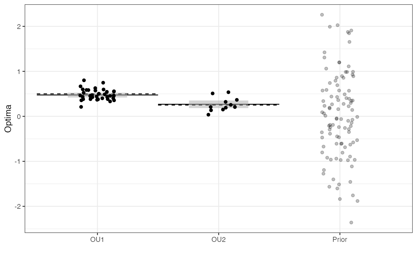

Next is the code for the Multilevel Multi-optima Model - here we include the additional prior sigma, which is a parameter for the variance among regimes

############################################################################################################
#Set Priors
hl.prior<-c(log(0.25),0.75)
vy.prior<-20
optima.prior<-c(0,1) #Informed by linear model
sigma.prior<-c(0,1)

############################################################################################################
#Blouch Prep Code
dat<-blouch.reg.mlm.prep(trdata,"Y_with_error","Y_error","regimes",hl.prior,vy.prior,optima.prior,sigma.prior)

fit.mlm.vi.regimes<- rstan::sampling(object = blouch:::stanmodels$blouchOU_reg_mlm_vi,data = dat,chains = 2,iter= 2000,cores=2)
#> Found more than one class "stanfit" in cache; using the first, from namespace 'rstan'
#> Also defined by 'rethinking'
#> Found more than one class "stanfit" in cache; using the first, from namespace 'rstan'
#> Also defined by 'rethinking'
#> Warning: There were 154 divergent transitions after warmup. See
#> https://mc-stan.org/misc/warnings.html#divergent-transitions-after-warmup
#> to find out why this is a problem and how to eliminate them.
#> Warning: Examine the pairs() plot to diagnose sampling problems

print(fit.mlm.vi.regimes,pars = c("hl","vy","optima","optima_bar","sigma"))
post<-rstan::extract(fit.mlm.vi.regimes)

Finally we will run the non-centered version of the same model, which can be used when the posterior is hard to explore and the centered version of the model produces divergences.

fit.mlm.vi.regimes.nc<- rstan::sampling(object = blouch:::stanmodels$blouchOU_reg_mlm_vi_nc,data = dat,chains = 2,iter =2000,cores=2) #,control=list(adapt_delta=0.95))
#> Found more than one class "stanfit" in cache; using the first, from namespace 'rstan'
#> Also defined by 'rethinking'
#> Found more than one class "stanfit" in cache; using the first, from namespace 'rstan'
#> Also defined by 'rethinking'
#> Warning: There were 74 divergent transitions after warmup. See
#> https://mc-stan.org/misc/warnings.html#divergent-transitions-after-warmup
#> to find out why this is a problem and how to eliminate them.
#> Warning: Examine the pairs() plot to diagnose sampling problems
#> Warning: Bulk Effective Samples Size (ESS) is too low, indicating posterior means and medians may be unreliable.
#> Running the chains for more iterations may help. See
#> https://mc-stan.org/misc/warnings.html#bulk-ess
#> Warning: Tail Effective Samples Size (ESS) is too low, indicating posterior variances and tail quantiles may be unreliable.
#> Running the chains for more iterations may help. See
#> https://mc-stan.org/misc/warnings.html#tail-ess
print(fit.mlm.vi.regimes.nc,pars = c("hl","vy","optima","optima_bar","sigma"))
###plot(rethinking::precis(fit.mlm.vi.regimes.nc,depth=2,pars = c("hl","vy","optima","optima_bar","sigma")))
post<-rstan::extract(fit.mlm.vi.regimes.nc)

rm(list=ls())

Multi-optima Direct Effect Model

We will now include both regimes painted on the tree and a direct effect predictor

############################################################################################################
#Regimes + Direct Effect Model
############################################################################################################
#Create phylogeny
########################################################################################################
N<-50 #Number of species
set.seed(10) #Set seed to get same random species each time

phy <- ape::keep.tip(tree.10K,sample(tree.10K$tip.label)[1:N]) 
phy<-ape::multi2di(phy)

l.tree<-max(ape::branching.times(phy)) ## rescale tree to height 1
phy$edge.length<-phy$edge.length/l.tree 

tip.label<-phy$tip.label

#Set regimes - manually - 2 regimes
#Locate nodes
plot(phy,no.margin=TRUE,edge.width=2,cex=0.7)
ape::nodelabels(frame="none",adj=c(1.1,-0.4))
ape::tiplabels()

#Paint Regimes on Tree
#source("/Users/markgrabowski/Documents/Academic/Research/Current Projects/Blouch project/blouch/Simulation Code/Functions/set.converge.regimes.R") #Macbook Pro
shifts<-c(84) #Location of nodes with regime shifts
trdata<-data.frame(phy$tip.label)
trdata<-treeplyr::make.treedata(phy,trdata)
trdata<-set.converge.regimes(trdata,shifts)
#> [1] 1
#>  [1] OU1 OU1 OU1 OU1 OU1 OU1 OU1 OU1 OU1 OU1 OU1 OU1 OU1 OU1 OU1 OU1 OU1 OU1 OU1
#> [20] OU1 OU1 OU1 OU1 OU1 OU1 OU1 OU1 OU1 OU1 OU1 OU1 OU1 OU1 OU1 OU1 OU1 OU1 OU1
#> [39] OU1 OU1 OU1 OU1 OU1 OU1 OU1 OU1 OU1 OU1 OU1 OU1 OU1 OU1 OU1 OU1 OU1 OU1 OU1
#> [58] OU1 OU1 OU1 OU1 OU1 OU1 OU1 OU2 OU2 OU2 OU2 OU2 OU2 OU2 OU2 OU2 OU2 OU2 OU2
#> [77] OU2 OU2 OU2 OU2 OU2 OU2 OU2 OU2 OU2 OU1 OU1 OU1 OU1 OU1 OU1 OU1 OU1 OU1 OU1
#> [96] OU1 OU1 OU1
#> Levels: OU1 OU2
#> [1] "#E64B35FF" "#4DBBD5FF"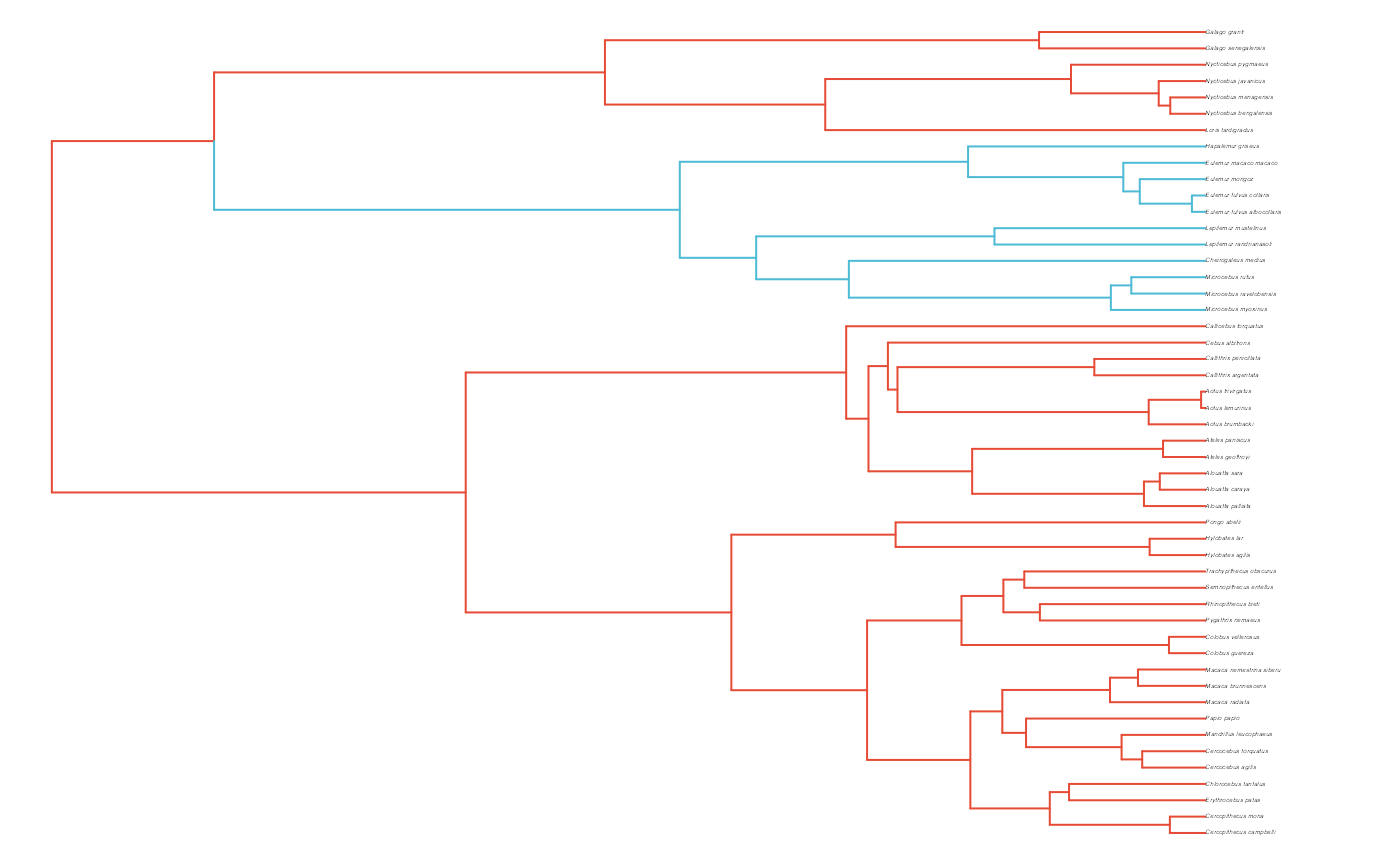

#Check if manual setting code worked
shifts.total<-c(trdata$dat$regimes,trdata$phy$node.label)
edge.regimes <- factor(shifts.total[trdata$phy$edge[,2]])
print(edge.regimes)
#>  [1] OU1 OU1 OU1 OU1 OU1 OU1 OU1 OU1 OU1 OU1 OU1 OU1 OU1 OU1 OU1 OU1 OU1 OU1 OU1
#> [20] OU1 OU1 OU1 OU1 OU1 OU1 OU1 OU1 OU1 OU1 OU1 OU1 OU1 OU1 OU1 OU1 OU1 OU1 OU1
#> [39] OU1 OU1 OU1 OU1 OU1 OU1 OU1 OU1 OU1 OU1 OU1 OU1 OU1 OU1 OU1 OU1 OU1 OU1 OU1
#> [58] OU1 OU1 OU1 OU1 OU1 OU1 OU1 OU2 OU2 OU2 OU2 OU2 OU2 OU2 OU2 OU2 OU2 OU2 OU2
#> [77] OU2 OU2 OU2 OU2 OU2 OU2 OU2 OU2 OU2 OU1 OU1 OU1 OU1 OU1 OU1 OU1 OU1 OU1 OU1
#> [96] OU1 OU1 OU1
#> Levels: OU1 OU2

reg.colors <- ggsci::pal_aaas("default", alpha = 0.7)(2)
print(reg.colors)
#> [1] "#3B4992B2" "#EE0000B2"
plot(trdata$phy,edge.color = reg.colors[edge.regimes], edge.width = 1, cex = 0.2)

#Phylogeny info
n<-length(trdata$phy$tip.label)
mrca1 <- ape::mrca(trdata$phy)
times <- ape::node.depth.edgelength(trdata$phy)

regimes_internal <-trdata$phy$node.label
regimes_tip <- trdata$dat$regimes
regimes <- concat.factor(regimes_tip, regimes_internal)
anc_maps<-"regimes"
lineages <- lapply(1:n, function(e) lineage.constructor(trdata$phy, e, anc_maps, regimes)) #Trace lineage from tips (n) to root and determine regimes of each node or branch

Now simulate X and Y data

#########################
hl<-0.1 #0.1, 0.25, 0.75 - testing options
a<-log(2)/hl
vy<-0.01 #0.25,0.5 - testing options
sigma2_y<-vy*(2*(log(2)/hl));

vX0<-0
vY0 <- 0
Sxx<-10 #Look at effects

Z_direct<-1

V<-calc_direct_V(phy,sigma2_y,a)
X<-phytools::fastBM(phy,a=vX0,sig2=Sxx,internal=FALSE) #Simulate X BM variable on tree, with scaling 10
#X<-rnorm(N,0,1)
names(X)<-phy$tip.label

phytools::phenogram(phy,X,spread.labels=TRUE,spread.cost=c(1,0)) #Plot X data
#> Optimizing the positions of the tip labels...

dmX<-weight.matrix(trdata$phy, a, lineages) #Slouch approach
dmX<-cbind(dmX,X)

beta<-c(2,1,0.25) #Two Optima/One Slope
mu<-dmX%*%beta #Simulate mu for Y

V<-calc_direct_V(phy,sigma2_y,a)
Y<-MASS::mvrnorm(n=1,mu,V)

#Plot data
df<-data.frame(Y=Y,X=X)

ggplot2::ggplot(data=df,ggplot2::aes(x=X,y=Y))+
  ggplot2::geom_point()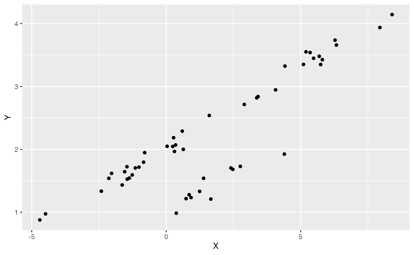

summary(lm(Y~X,df))
#> 
#> Call:
#> lm(formula = Y ~ X, data = df)
#> 
#> Residuals:
#>      Min       1Q   Median       3Q      Max 
#> -1.00801  0.05843  0.18122  0.26742  0.44140 
#> 
#> Coefficients:
#>             Estimate Std. Error t value Pr(>|t|)    
#> (Intercept)  1.79802    0.07104   25.31   <2e-16 ***
#> X            0.25223    0.02025   12.46   <2e-16 ***
#> ---
#> Signif. codes:  0 '***' 0.001 '**' 0.01 '*' 0.05 '.' 0.1 ' ' 1
#> 
#> Residual standard error: 0.4464 on 48 degrees of freedom
#> Multiple R-squared:  0.7638, Adjusted R-squared:  0.7589 
#> F-statistic: 155.2 on 1 and 48 DF,  p-value: < 2.2e-16

#################################################################################################################Simulate errors
Z_X_error<-1 #Number of X traits with error
X_error<-rep(0.01,N)
Y_error<-rep(0.01,N)
Y_with_error<-Y+rnorm(N,0,0.01)
X_with_error<-X+rnorm(N,0,0.01)

############################################################################################################
#Make trdata file
trdata$dat<-cbind(trdata$dat,data.frame(cbind(Y_with_error,Y_error,X_with_error,X_error)))

Next we will set the priors for the estimated parameters - for this model this includes the half-life, Vy, optima, and beta. For the latter two parameters we will use the results of the linear model to inform our priors.

############################################################################################################
#Set Priors
hl.prior<-c(log(0.25),0.75)
vy.prior<-5
optima.prior<-c(2,0.5) #Informed by linear model
beta.prior<-c(0.25,0.25) #Informed by linear model

Exploring Priors

At this point one would want to explore if the priors are appropriate - do the prior distributions look consistent with what we know about our system? See Grabowski (in press) for more on setting priors.

Half-life Prior plot

hl.sims<-data.frame(rlnorm(n=1000,meanlog=hl.prior[1],sdlog=hl.prior[2]))
names(hl.sims)<-"prior.hl.sims"

hl.prior.plot<-ggplot2::ggplot()+
  ggplot2::geom_density(ggplot2::aes(prior.hl.sims,fill="prior.hl.sims"),alpha=0.2,data=hl.sims)+
  ggplot2::theme_bw()+
  ggplot2::theme(
    panel.grid.major = ggplot2::element_blank(),
    panel.grid.minor = ggplot2::element_blank())+
  
  #labs(title="Prior vs. Posterior Distribution ",x="Half-life", y = "Density")+
  ggplot2::labs(title="",x="Half-life", y = "Density")+
  
  #scale_fill_manual(labels=c("Posterior","Prior"))+
  ggplot2::geom_vline(xintercept=c(hl),linetype=2)+
  ggsci::scale_fill_npg(name="",labels=c("Prior"))

hl.prior.plot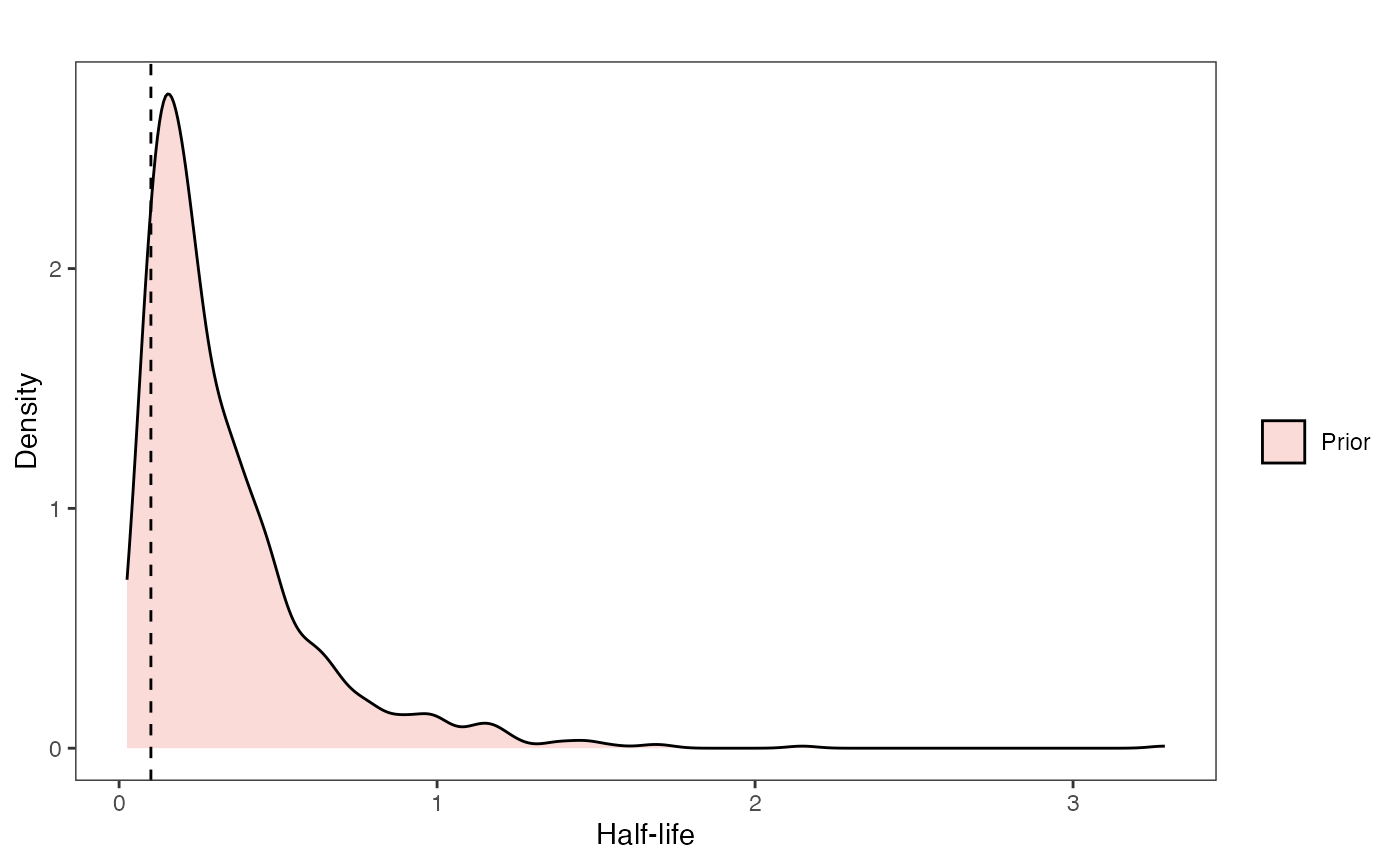

Vy Prior Plot

vy.sims<-rexp(n=1000,rate=vy.prior)
vy.sims<-data.frame(vy.sims)
names(vy.sims)<-"prior.vy.sims"

vy.prior.plot<-ggplot2::ggplot()+
  ggplot2::geom_density(ggplot2::aes(prior.vy.sims,fill="prior.vy.sims"),alpha=0.2,data=vy.sims)+
  ggplot2::theme_bw()+
  ggplot2::theme(
    panel.grid.major = ggplot2::element_blank(),
    panel.grid.minor = ggplot2::element_blank())+
  
  #labs(title="Prior vs. Posterior Distribution ",x="vy", y = "Density")+
  ggplot2::labs(title="",x="vy", y = "Density")+
  ggplot2::geom_vline(xintercept=c(vy),linetype=2)+
  
  #scale_fill_manual(labels=c("Posterior","Prior"))+
  ggsci::scale_fill_npg(name="",labels=c("Prior"))


vy.prior.plot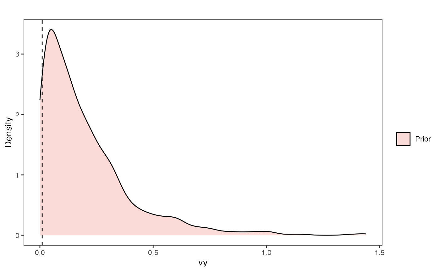

Prior on how shared branch lengths correspond to covariance

a.sims<-log(2)/hl.sims;
sigma2_y.sims<-vy.sims*(2*(log(2)/hl.sims));
#x<-seq(from=0,to=1,by=0.001)
#V.sim<-calc_direct_V(phy,a.sims,sigma2_y.sims)

plot( NULL , xlim=c(0,1) , ylim=c(0,1) , xlab="Time since MRCA" , ylab="Covariance" ,cex.axis=0.75, mgp=c(1.25,0.25,0),tcl=-0.25)
for (i in 1:30){
  curve(sigma2_y.sims[i,] /(2 * a.sims[i,]) * ((1 - exp(-2 * a.sims[i,] * (1-(x/2)))) * exp(-a.sims[i,] * x)) , add=TRUE , lwd=4 , col=rethinking::col.alpha(1,0.15))
}

par(mar=c(3,3,0.25,0.25))
covariance.prior.plot <- recordPlot()
dev.off()
#> null device 
#>           1
covariance.prior.plot

Slope and intercept Prior Plot

optima.sims<-rnorm(100,optima.prior[1],optima.prior[2])
beta.sims<-rnorm(n=100,beta.prior[1],beta.prior[2])

prior.slope.plot<-ggplot2::ggplot()+  
 ggplot2:: geom_point(data=df,ggplot2::aes(y=Y,x=X))+
  ggplot2::geom_abline(intercept=optima.sims,slope=beta.sims,alpha=0.15)+
  ggplot2::theme_bw()+
  ggplot2::theme(
    panel.grid.major = ggplot2::element_blank(),
    panel.grid.minor = ggplot2::element_blank())+
  
  ggplot2::ylab("Y") + ggplot2::xlab("Direct Effect X")+
  ggsci::scale_color_npg()

prior.slope.plot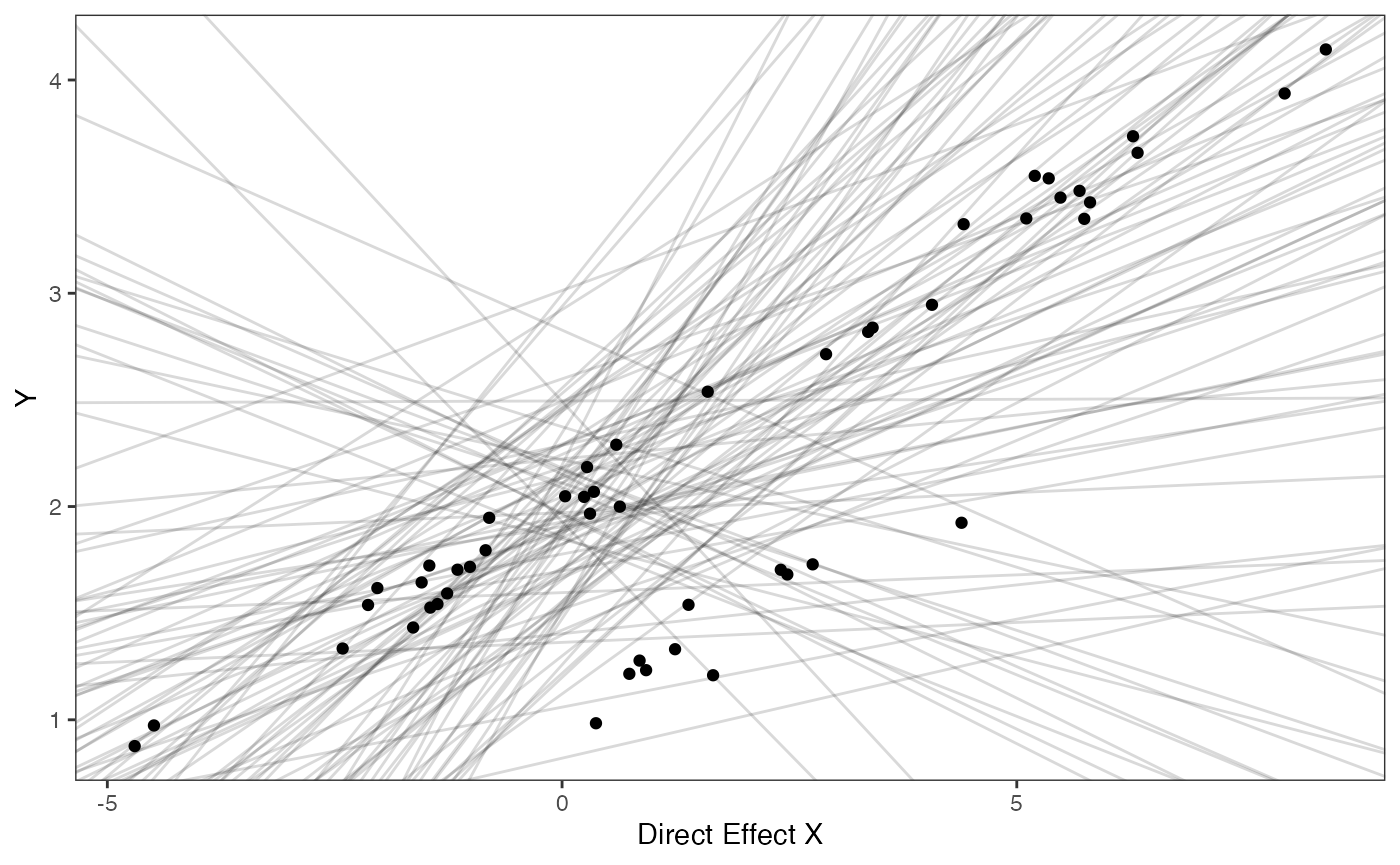

We will use the helper function blouch.reg.direct.prep() to setup the dat file for Stan. Here “Z_direct” is the number of predictors, and “regimes” is the name of the regime column in trdata$dat.

############################################################################################################
#Test Blouch prep code - Regimes + Direct Efffect model
dat<-blouch.reg.direct.prep(trdata,"Y_with_error","Y_error","X_with_error","X_error",Z_direct=1,"regimes",hl.prior,vy.prior,optima.prior,beta.prior)

Now we run the basic Multi-optima Direct Effect Model, look at the results, and rstan::extract the posterior

fit.reg.direct<- rstan::sampling(object = blouch:::stanmodels$blouchOU_reg_direct,data = dat,chains = 2,cores=2,iter=2000)
#> Found more than one class "stanfit" in cache; using the first, from namespace 'rstan'
#> Also defined by 'rethinking'
#> Found more than one class "stanfit" in cache; using the first, from namespace 'rstan'
#> Also defined by 'rethinking'

print(fit.reg.direct,pars = c("hl","vy","optima","beta"))
#> Inference for Stan model: blouchOU_reg_direct.
#> 2 chains, each with iter=2000; warmup=1000; thin=1; 
#> post-warmup draws per chain=1000, total post-warmup draws=2000.
#> 
#>           mean se_mean   sd 2.5%  25%  50%  75% 97.5% n_eff Rhat
#> hl        0.16       0 0.08 0.06 0.11 0.15 0.20  0.36  1153    1
#> vy        0.02       0 0.01 0.01 0.01 0.02 0.02  0.03  1334    1
#> optima[1] 2.01       0 0.04 1.93 1.99 2.01 2.04  2.09  2807    1
#> optima[2] 0.94       0 0.09 0.73 0.90 0.95 0.99  1.07  1158    1
#> beta[1]   0.25       0 0.01 0.24 0.25 0.25 0.26  0.27  2788    1
#> 
#> Samples were drawn using NUTS(diag_e) at Tue Oct  8 13:47:40 2024.
#> For each parameter, n_eff is a crude measure of effective sample size,
#> and Rhat is the potential scale reduction factor on split chains (at 
#> convergence, Rhat=1).
post<-rstan::extract(fit.reg.direct) #rstan::extract posterior distribution

Now lets look at the prior vs. posterior plots for the parameters Half-life plot

hl.post<-data.frame(post$hl)
names(hl.post)<-"post.hl.sims"

hl.plot<-ggplot2::ggplot()+
  ggplot2::geom_density(ggplot2::aes(prior.hl.sims,fill="prior.hl.sims"),alpha=0.2,data=hl.sims)+
  ggplot2::geom_density(ggplot2::aes(post.hl.sims,fill="post.hl.sims"),alpha=0.2,data=hl.post)+
  ggplot2::theme_bw()+
  ggplot2::theme(
    panel.grid.major = ggplot2::element_blank(),
    panel.grid.minor = ggplot2::element_blank())+
  
  #labs(title="Prior vs. Posterior Distribution ",x="Half-life", y = "Density")+
  ggplot2::labs(title="",x="Half-life", y = "Density")+
  
  #scale_fill_manual(labels=c("Posterior","Prior"))+
  ggplot2::geom_vline(xintercept=c(hl),linetype=2)+
  ggsci::scale_fill_npg(name="",labels=c("Posterior","Prior"))

hl.plot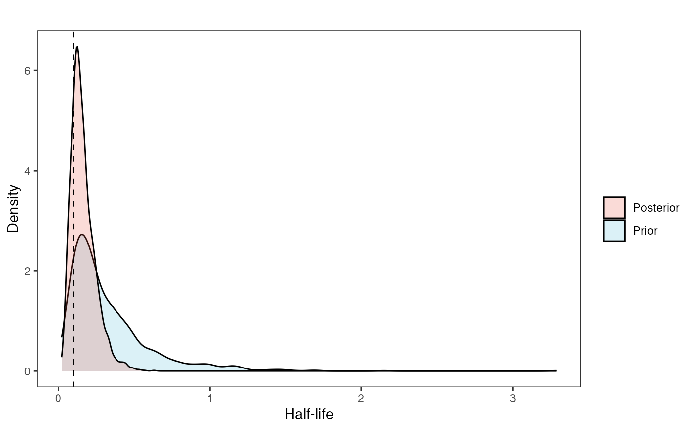

Vy Prior vs. posterior plot

vy.post<-data.frame(post$vy)
names(vy.post)<-"post.vy.sims"


vy.plot<-ggplot2::ggplot()+
  ggplot2::geom_density(ggplot2::aes(prior.vy.sims,fill="prior.vy.sims"),alpha=0.2,data=vy.sims)+
  ggplot2::geom_density(ggplot2::aes(post.vy.sims,fill="post.vy.sims"),alpha=0.2,data=vy.post)+
  ggplot2::theme_bw()+
  ggplot2::theme(
    panel.grid.major = ggplot2::element_blank(),
    panel.grid.minor = ggplot2::element_blank())+
  
  #labs(title="Prior vs. Posterior Distribution ",x="vy", y = "Density")+
  ggplot2::labs(title="",x="vy", y = "Density")+
  ggplot2::geom_vline(xintercept=c(vy),linetype=2)+
  
  #scale_fill_manual(labels=c("Posterior","Prior"))+
  ggsci::scale_fill_npg(name="",labels=c("Posterior","Prior"))

vy.plot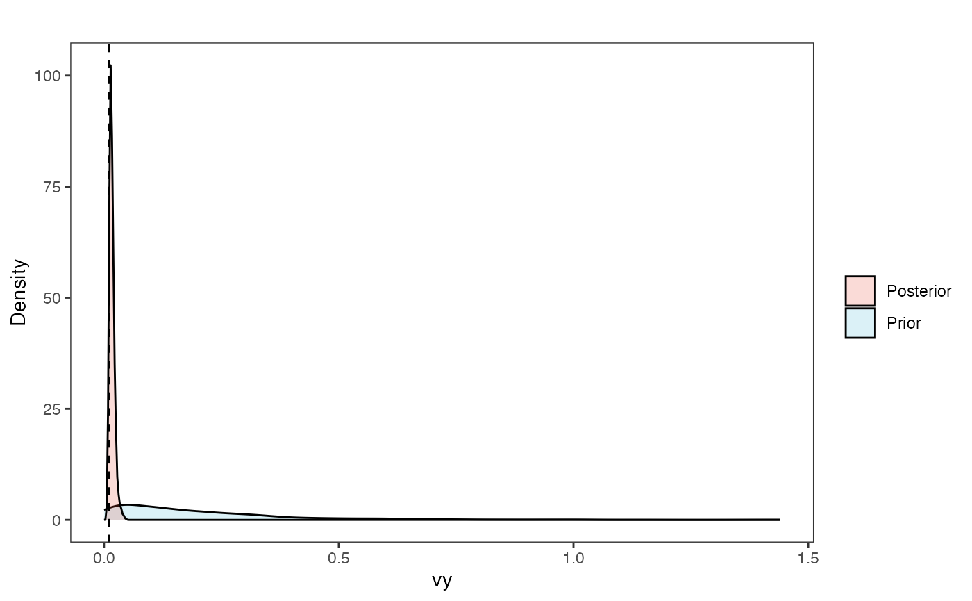

Prior versus posterior on how shared branch lengths correspond to covariance

plot( NULL , xlim=c(0,1) , ylim=c(0,1) , xlab="Time since MRCA" , ylab="Covariance" ,cex.axis=0.75, mgp=c(1.25,0.25,0),tcl=-0.25)
for (i in 1:30){
  curve(sigma2_y.sims[i,] /(2 * a.sims[i,]) * ((1 - exp(-2 * a.sims[i,] * (1-(x/2)))) * exp(-a.sims[i,] * x)) , add=TRUE , lwd=4 , col=rethinking::col.alpha(1,0.15))
}

for (i in 1:30){
  curve(post$sigma2_y[i] /(2 * post$a[i]) * ((1 - exp(-2 * post$a[i] * (1-(x/2)))) * exp(-post$a[i] * x)) , add=TRUE , lwd=4 , col=rethinking::col.alpha(2,0.5))
}

par(mar=c(3,3,0.25,0.25))
covariance.plot <- recordPlot()
dev.off()
#> null device 
#>           1
covariance.plot

Prior vs. Posterior Plot for Regression

optima.sims<-rnorm(100,optima.prior[1],optima.prior[2])
beta.sims<-rnorm(n=100,beta.prior[1],beta.prior[2])

optima.post<-post$optima
beta.post<-data.frame(post$beta)
names(beta.post)<-c("post.beta.1")

mu.link.11<-function(x.seq){optima.post[,1]+x.seq*beta.post[,1]}
mu.link.12<-function(x.seq){optima.post[,2]+x.seq*beta.post[,1]}

x.seq <- seq(from=min(X), to=max(X) , length.out=100)
mu.11 <- sapply(x.seq , mu.link.11 )
mu.12 <- sapply(x.seq , mu.link.12 )


mu.mean.11<-colMeans(mu.11)
mu.mean.12<-colMeans(mu.12)

mu.mean.11<-data.frame(as.numeric(mu.mean.11))
mu.mean.12<-data.frame(as.numeric(mu.mean.12))

names(mu.mean.11)<-"mu.mean.11"
names(mu.mean.12)<-"mu.mean.12"

mu.CI.11 <- apply( mu.11 , MARGIN=2, FUN=rethinking::PI , prob=0.89 )
mu.CI.12 <- apply( mu.12 , MARGIN=2, FUN=rethinking::PI , prob=0.89 )


mu.CI.11<-data.frame(t(data.frame(mu.CI.11)),x.seq)
mu.CI.12<-data.frame(t(data.frame(mu.CI.12)),x.seq)

names(mu.CI.11)<-c("min.5.5","max.94.5","x.seq")
names(mu.CI.12)<-c("min.5.5","max.94.5","x.seq")

#df<-data.frame(Y=stan_sim_data$Y,X=stan_sim_data$direct_cov)
df<-data.frame(Y=dat$Y_obs,X=dat$X_obs,Regimes=regimes_tip)
df11<-data.frame(x.seq,mu.mean.11)
df12<-data.frame(x.seq,mu.mean.12)

#slope.prior.plot<-ggplot(data=reg.trdata$dat,aes(y=Sim1,x=X))+
slope.plot.1<-ggplot2::ggplot()+  
  ggplot2::geom_point(data=df,ggplot2::aes(y=Y,x=X,color=as.factor(Regimes)))+
  ggplot2::geom_abline(intercept=optima.sims,slope=beta.sims,alpha=0.05)+ #Prior
  ggplot2::geom_abline(intercept=beta[1],slope=beta[3],alpha=0.5,linetype=2)+
  ggplot2::geom_abline(intercept=beta[2],slope=beta[3],alpha=0.5,linetype=2)+
  ggplot2::geom_ribbon(data=mu.CI.11,ggplot2::aes(x=x.seq,ymin=min.5.5,ymax=max.94.5),linetype=2,alpha=0.1)+
  ggplot2::geom_line(data=df11,ggplot2::aes(x=x.seq,y=mu.mean.11),linetype=1,linewidth=1,alpha=0.3)+
  ggplot2::geom_ribbon(data=mu.CI.12,ggplot2::aes(x=x.seq,ymin=min.5.5,ymax=max.94.5),linetype=2,alpha=0.1)+
  ggplot2::geom_line(data=df12,ggplot2::aes(x=x.seq,y=mu.mean.12),linetype=1,linewidth=1,alpha=0.3)+
  ggplot2::theme_bw()+
  ggplot2::theme(
    panel.grid.major = ggplot2::element_blank(),
    panel.grid.minor = ggplot2::element_blank())+
  
  #ggtitle("Prior vs. Posterior for Intercept and Slope")+
  ggplot2::ylab("Y") + ggplot2::xlab("Direct Effect X")+ggplot2::labs(color="Regimes")+
  ggsci::scale_color_npg()

slope.plot.1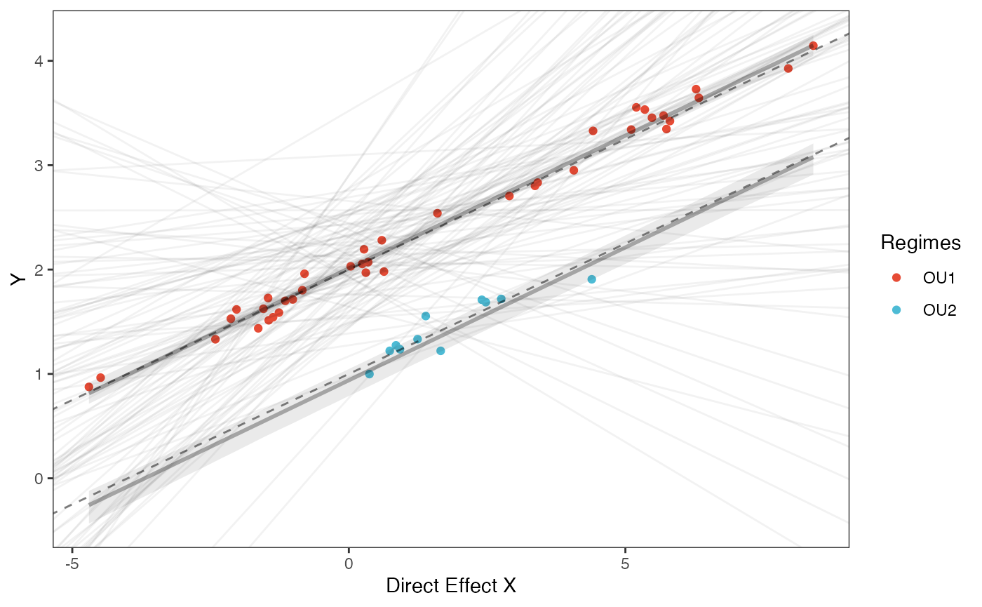

#Label points

Here is the Multilevel version of the same model

############################################################################################################
#Set Priors
hl.prior<-c(log(0.25),0.75)
vy.prior<-5
optima.prior<-c(2,0.5) #Informed by linear model
beta.prior<-c(0.25,0.25) #Informed by linear model
sigma.prior<-c(0,1)

We will use the helper function blouch.reg.direct.prep() to setup the dat file for Stan. Here “Z_direct” is the number of predictors, and “regimes” is the name of the regime column in trdata$dat.

############################################################################################################
#Test Blouch prep code - Regimes + Direct Efffect model
dat<-blouch.reg.direct.mlm.prep(trdata,"Y_with_error","Y_error","X_with_error","X_error",Z_direct=1,"regimes",hl.prior,vy.prior,optima.prior,beta.prior,sigma.prior)

fit.reg.direct.mlm.vi<- rstan::sampling(object = blouch:::stanmodels$blouchOU_reg_direct_mlm_vi,data = dat,chains = 2,cores=2,iter = 2000)
#> Found more than one class "stanfit" in cache; using the first, from namespace 'rstan'
#> Also defined by 'rethinking'
#> Found more than one class "stanfit" in cache; using the first, from namespace 'rstan'
#> Also defined by 'rethinking'

print(fit.reg.direct.mlm.vi,pars = c("hl","vy","optima","optima_bar","beta","sigma"))
#> Inference for Stan model: blouchOU_reg_direct_mlm_vi.
#> 2 chains, each with iter=2000; warmup=1000; thin=1; 
#> post-warmup draws per chain=1000, total post-warmup draws=2000.
#> 
#>            mean se_mean   sd 2.5%  25%  50%  75% 97.5% n_eff Rhat
#> hl         0.17    0.00 0.10 0.06 0.11 0.15 0.21  0.45   701    1
#> vy         0.02    0.00 0.01 0.01 0.01 0.02 0.02  0.04   666    1
#> optima[1]  2.01    0.00 0.04 1.93 1.99 2.01 2.03  2.09  2407    1
#> optima[2]  0.92    0.00 0.11 0.62 0.88 0.94 0.99  1.05   732    1
#> optima_bar 1.76    0.01 0.38 1.05 1.51 1.74 2.00  2.57  3375    1
#> beta[1]    0.25    0.00 0.01 0.24 0.25 0.25 0.26  0.27  3129    1
#> sigma      0.90    0.01 0.42 0.32 0.60 0.82 1.12  1.96  2388    1
#> 
#> Samples were drawn using NUTS(diag_e) at Tue Oct  8 13:48:02 2024.
#> For each parameter, n_eff is a crude measure of effective sample size,
#> and Rhat is the potential scale reduction factor on split chains (at 
#> convergence, Rhat=1).
post<-rstan::extract(fit.reg.direct.mlm.vi) #rstan::extract posterior distribution

And finally the non-centered version of the Multilevel model

fit.reg.direct.mlm.vi<- rstan::sampling(object = blouch:::stanmodels$blouchOU_reg_direct_mlm_vi_nc,data = dat,chains = 2,cores=2,iter = 2000)
#> Found more than one class "stanfit" in cache; using the first, from namespace 'rstan'
#> Also defined by 'rethinking'
#> Found more than one class "stanfit" in cache; using the first, from namespace 'rstan'
#> Also defined by 'rethinking'
#> Warning: There were 193 divergent transitions after warmup. See
#> https://mc-stan.org/misc/warnings.html#divergent-transitions-after-warmup
#> to find out why this is a problem and how to eliminate them.
#> Warning: Examine the pairs() plot to diagnose sampling problems
#> Warning: The largest R-hat is NA, indicating chains have not mixed.
#> Running the chains for more iterations may help. See
#> https://mc-stan.org/misc/warnings.html#r-hat
#> Warning: Bulk Effective Samples Size (ESS) is too low, indicating posterior means and medians may be unreliable.
#> Running the chains for more iterations may help. See
#> https://mc-stan.org/misc/warnings.html#bulk-ess
#> Warning: Tail Effective Samples Size (ESS) is too low, indicating posterior variances and tail quantiles may be unreliable.
#> Running the chains for more iterations may help. See
#> https://mc-stan.org/misc/warnings.html#tail-ess

print(fit.reg.direct.mlm.vi,pars = c("hl","vy","optima","optima_bar","beta","sigma"))
#> Inference for Stan model: blouchOU_reg_direct_mlm_vi_nc.
#> 2 chains, each with iter=2000; warmup=1000; thin=1; 
#> post-warmup draws per chain=1000, total post-warmup draws=2000.
#> 
#>            mean se_mean   sd 2.5%  25%  50%  75% 97.5% n_eff Rhat
#> hl         0.17    0.01 0.10 0.06 0.10 0.15 0.21  0.44   200 1.01
#> vy         0.02    0.00 0.01 0.01 0.01 0.02 0.02  0.03   503 1.00
#> optima[1]  2.01    0.00 0.04 1.92 1.99 2.01 2.03  2.09  1977 1.00
#> optima[2]  0.92    0.00 0.12 0.59 0.89 0.94 0.98  1.06   927 1.00
#> optima_bar 1.81    0.05 0.40 1.07 1.53 1.77 2.08  2.58    74 1.03
#> beta[1]    0.26    0.00 0.01 0.24 0.25 0.26 0.26  0.27  1114 1.01
#> sigma      0.97    0.08 0.48 0.34 0.61 0.86 1.21  2.11    33 1.06
#> 
#> Samples were drawn using NUTS(diag_e) at Tue Oct  8 13:49:07 2024.
#> For each parameter, n_eff is a crude measure of effective sample size,
#> and Rhat is the potential scale reduction factor on split chains (at 
#> convergence, Rhat=1).
post<-rstan::extract(fit.reg.direct.mlm.vi) #rstan::extract posterior distribution

rm(list=ls())

Multi-optima Adaptive Model

We will now include both regimes painted on the tree and an adaptive predictor

#Create phylogeny
########################################################################################################
N<-50 #Number of species
set.seed(10) #Set seed to get same random species each time

phy <- ape::keep.tip(tree.10K,sample(tree.10K$tip.label)[1:N]) 
phy<-ape::multi2di(phy)

l.tree<-max(ape::branching.times(phy)) ## rescale tree to height 1
phy$edge.length<-phy$edge.length/l.tree 

tip.label<-phy$tip.label

#Set regimes - manually - 2 regimes
#Locate nodes
plot(phy,no.margin=TRUE,edge.width=2,cex=0.7)
ape::nodelabels(frame="none",adj=c(1.1,-0.4))
ape::tiplabels()

#Paint Regimes on Tree
shifts<-c(84) #Location of nodes with regime shifts
trdata<-data.frame(phy$tip.label)
trdata<-treeplyr::make.treedata(phy,trdata)
trdata<-set.converge.regimes(trdata,shifts)
#> [1] 1
#>  [1] OU1 OU1 OU1 OU1 OU1 OU1 OU1 OU1 OU1 OU1 OU1 OU1 OU1 OU1 OU1 OU1 OU1 OU1 OU1
#> [20] OU1 OU1 OU1 OU1 OU1 OU1 OU1 OU1 OU1 OU1 OU1 OU1 OU1 OU1 OU1 OU1 OU1 OU1 OU1
#> [39] OU1 OU1 OU1 OU1 OU1 OU1 OU1 OU1 OU1 OU1 OU1 OU1 OU1 OU1 OU1 OU1 OU1 OU1 OU1
#> [58] OU1 OU1 OU1 OU1 OU1 OU1 OU1 OU2 OU2 OU2 OU2 OU2 OU2 OU2 OU2 OU2 OU2 OU2 OU2
#> [77] OU2 OU2 OU2 OU2 OU2 OU2 OU2 OU2 OU2 OU1 OU1 OU1 OU1 OU1 OU1 OU1 OU1 OU1 OU1
#> [96] OU1 OU1 OU1
#> Levels: OU1 OU2
#> [1] "#E64B35FF" "#4DBBD5FF"

#Check if manual setting code worked
shifts.total<-c(trdata$dat$regimes,trdata$phy$node.label)
edge.regimes <- factor(shifts.total[trdata$phy$edge[,2]])
print(edge.regimes)
#>  [1] OU1 OU1 OU1 OU1 OU1 OU1 OU1 OU1 OU1 OU1 OU1 OU1 OU1 OU1 OU1 OU1 OU1 OU1 OU1
#> [20] OU1 OU1 OU1 OU1 OU1 OU1 OU1 OU1 OU1 OU1 OU1 OU1 OU1 OU1 OU1 OU1 OU1 OU1 OU1
#> [39] OU1 OU1 OU1 OU1 OU1 OU1 OU1 OU1 OU1 OU1 OU1 OU1 OU1 OU1 OU1 OU1 OU1 OU1 OU1
#> [58] OU1 OU1 OU1 OU1 OU1 OU1 OU1 OU2 OU2 OU2 OU2 OU2 OU2 OU2 OU2 OU2 OU2 OU2 OU2
#> [77] OU2 OU2 OU2 OU2 OU2 OU2 OU2 OU2 OU2 OU1 OU1 OU1 OU1 OU1 OU1 OU1 OU1 OU1 OU1
#> [96] OU1 OU1 OU1
#> Levels: OU1 OU2

reg.colors <- ggsci::pal_aaas("default", alpha = 0.7)(2)
print(reg.colors)
#> [1] "#3B4992B2" "#EE0000B2"
plot(trdata$phy,edge.color = reg.colors[edge.regimes], edge.width = 1, cex = 0.2)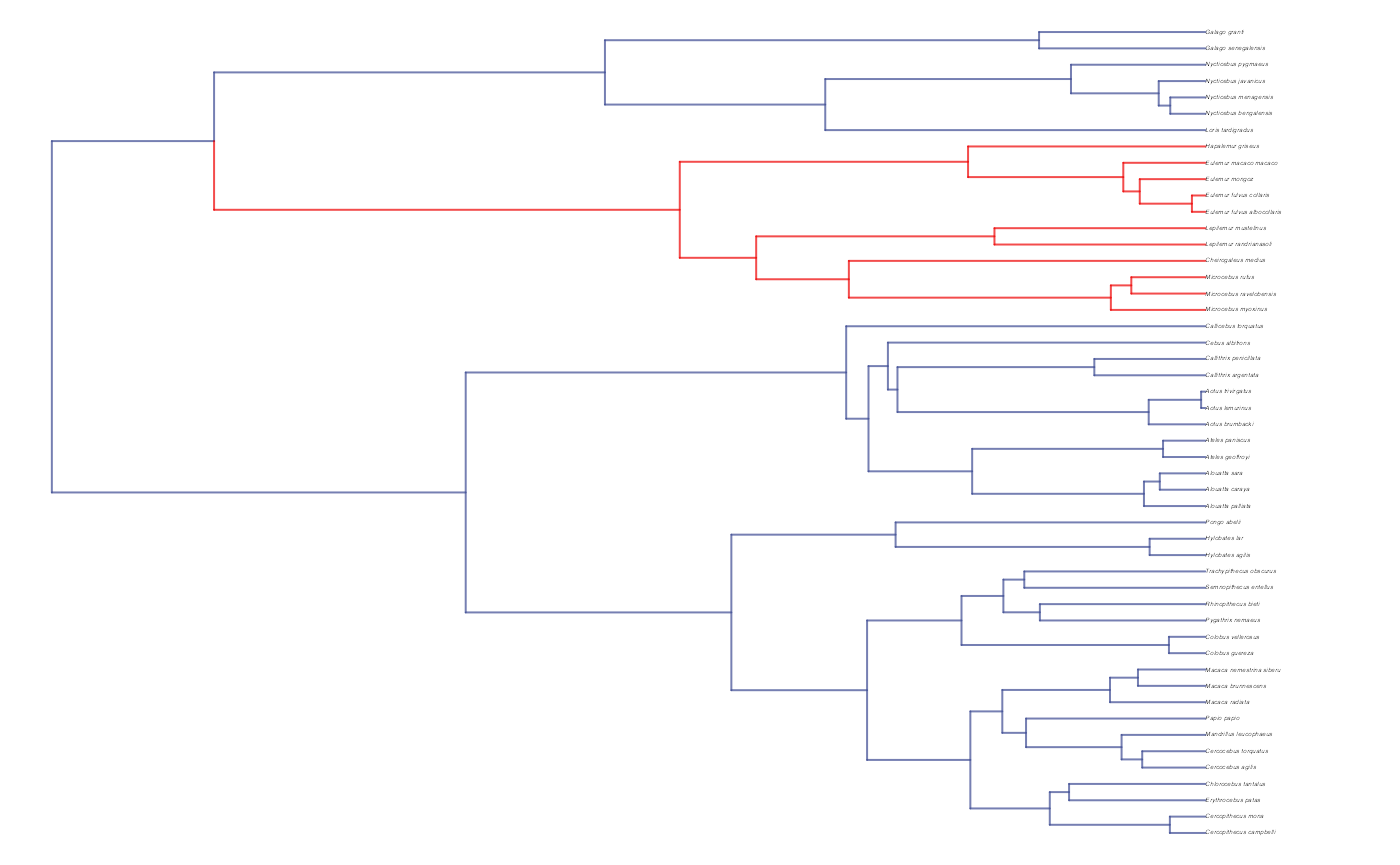

#Phylogeny info
n<-length(trdata$phy$tip.label)

regimes_internal <-trdata$phy$node.label
regimes_tip <- trdata$dat$regimes
regimes <- concat.factor(regimes_tip, regimes_internal)
anc_maps<-"regimes"
lineages <- lapply(1:n, function(e) lineage.constructor(trdata$phy, e, anc_maps, regimes)) #Trace lineage from tips (n) to root and determine regimes of each node or branch

Simulate X and Y data using generative model

############################################################################################################
#########################
hl<-0.1 #0.1, 0.25, 0.75 - testing options
a<-log(2)/hl
vy<-0.01 #0.25,0.5 - testing options
sigma2_y<-vy*(2*(log(2)/hl));

vX0<-0
vY0 <- 0

Z_adaptive<-1
sigma2_x<-matrix(1,1,1) #Variance of BM Process

X<-phytools::fastBM(phy,a=vX0,sig2=sigma2_x[1,1],internal=FALSE) #Simulate X BM variable on tree, with scaling 10
phytools::phenogram(phy,X,spread.labels=TRUE,spread.cost=c(1,0)) #Plot X data
#> Optimizing the positions of the tip labels...

#sigma2_x<-ratematrix(phy,Xa) #Calculate evolutionary v/cv matrix

dmX<-weight.matrix(trdata$phy, a, lineages) #Slouch approach
dmX<-cbind(dmX,calc_adaptive_dmX(phy,a,X))

beta<-c(2,1,0.25) #Two Optima/Two Slopes
mu<-dmX%*%beta #Simulate mu for Y

V<-calc_adaptive_V(phy,a, sigma2_y, beta[3],  sigma2_x,Z_adaptive)
Y<-MASS::mvrnorm(n=1,mu,V)

################################################################################################################
#Plot data
df<-data.frame(Y=Y,X=X)

ggplot2::ggplot(data=df,ggplot2::aes(x=X,y=Y))+
  ggplot2::geom_point()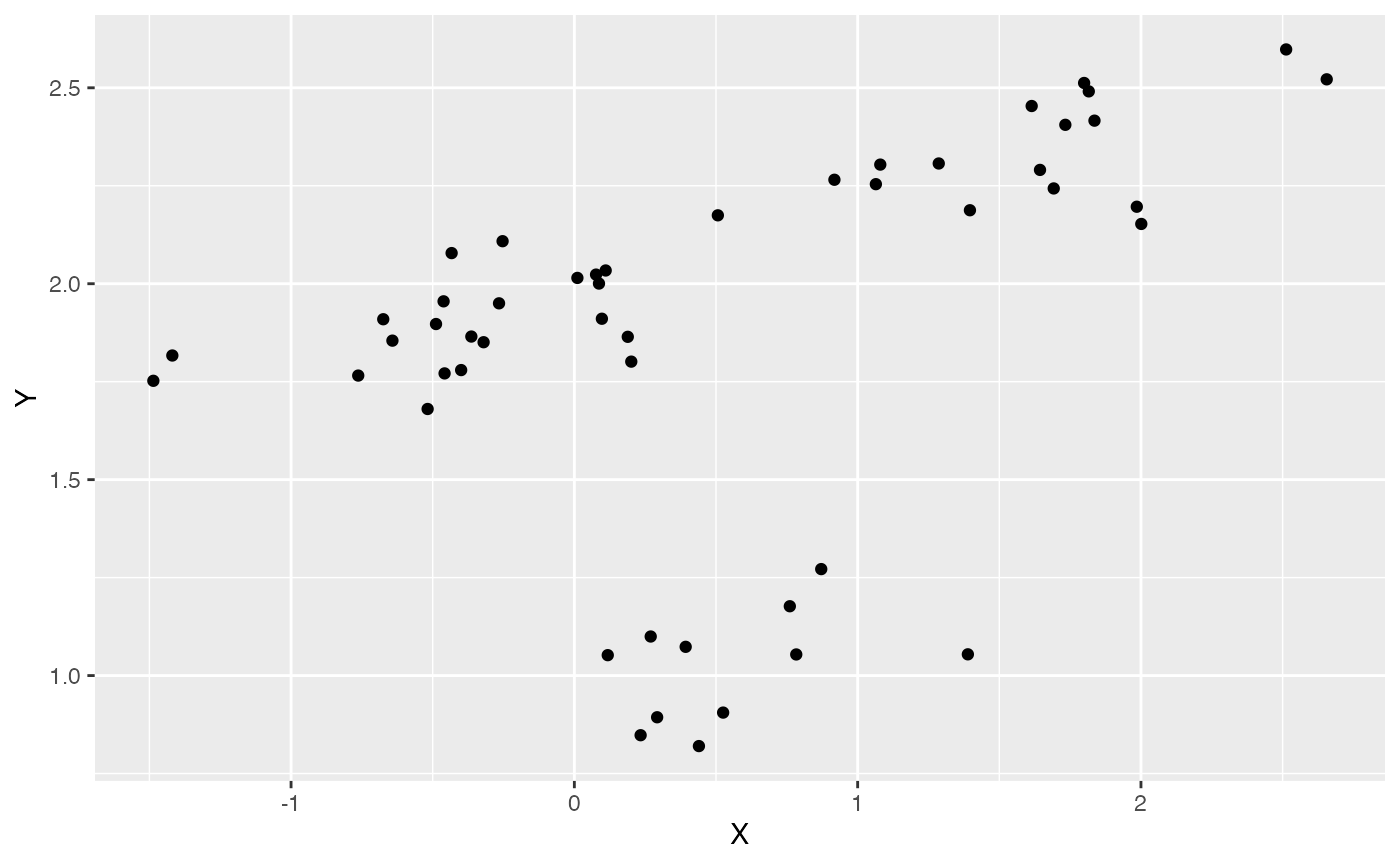

summary(lm(Y~X,df))
#> 
#> Call:
#> lm(formula = Y ~ X, data = df)
#> 
#> Residuals:
#>     Min      1Q  Median      3Q     Max 
#> -1.0206  0.0130  0.2201  0.2994  0.4077 
#> 
#> Coefficients:
#>             Estimate Std. Error t value Pr(>|t|)    
#> (Intercept)  1.75536    0.07480  23.467  < 2e-16 ***
#> X            0.19407    0.06742   2.879  0.00595 ** 
#> ---
#> Signif. codes:  0 '***' 0.001 '**' 0.01 '*' 0.05 '.' 0.1 ' ' 1
#> 
#> Residual standard error: 0.47 on 48 degrees of freedom
#> Multiple R-squared:  0.1472, Adjusted R-squared:  0.1295 
#> F-statistic: 8.287 on 1 and 48 DF,  p-value: 0.005947
################################################################################################################
#Simulate errors
Z_X_error<-1 #Number of X traits with error
X_error<-rep(0.01,N)
Y_error<-rep(0.01,N)
Y_with_error<-Y+rnorm(N,0,0.01)
X_with_error<-X+rnorm(N,0,0.01)

############################################################################################################
#Make trdata file
trdata$dat<-cbind(trdata$dat,data.frame(cbind(Y_with_error,Y_error,X_with_error,X_error)))
############################################################################################################

Next we will set the priors for the estimated parameters - for this model this includes the half-life, Vy, optima, and beta. For the latter two parameters we will use the results of the linear model to inform our priors.

############################################################################################################
#Set Priors
hl.prior<-c(log(0.25),0.75)
vy.prior<-5
optima.prior<-c(1.75,0.55) #Informed by linear model
beta.prior<-c(0.25,0.25) #Informed by linear model

Exploring Priors

At this point one would want to explore if the priors are appropriate - do the prior distributions look consistent with what we know about our system? See Grabowski (in press) for more on setting priors.

Half-life Prior plot

hl.sims<-data.frame(rlnorm(n=1000,meanlog=hl.prior[1],sdlog=hl.prior[2]))
names(hl.sims)<-"prior.hl.sims"

hl.prior.plot<-ggplot2::ggplot()+
  ggplot2::geom_density(ggplot2::aes(prior.hl.sims,fill="prior.hl.sims"),alpha=0.2,data=hl.sims)+
  ggplot2::theme_bw()+
  ggplot2::theme(
    panel.grid.major = ggplot2::element_blank(),
    panel.grid.minor = ggplot2::element_blank())+
  
  #labs(title="Prior vs. Posterior Distribution ",x="Half-life", y = "Density")+
  ggplot2::labs(title="",x="Half-life", y = "Density")+
  
  #scale_fill_manual(labels=c("Posterior","Prior"))+
  ggplot2::geom_vline(xintercept=c(hl),linetype=2)+
  ggsci::scale_fill_npg(name="",labels=c("Prior"))

hl.prior.plot

Vy Prior Plot

vy.sims<-rexp(n=1000,rate=vy.prior)
vy.sims<-data.frame(vy.sims)
names(vy.sims)<-"prior.vy.sims"

vy.prior.plot<-ggplot2::ggplot()+
  ggplot2::geom_density(ggplot2::aes(prior.vy.sims,fill="prior.vy.sims"),alpha=0.2,data=vy.sims)+
  ggplot2::theme_bw()+
  ggplot2::theme(
    panel.grid.major = ggplot2::element_blank(),
    panel.grid.minor = ggplot2::element_blank())+
  
  #labs(title="Prior vs. Posterior Distribution ",x="vy", y = "Density")+
  ggplot2::labs(title="",x="vy", y = "Density")+
  ggplot2::geom_vline(xintercept=c(vy),linetype=2)+
  
  #scale_fill_manual(labels=c("Posterior","Prior"))+
  ggsci::scale_fill_npg(name="",labels=c("Prior"))


vy.prior.plot

Prior on how shared branch lengths correspond to covariance

a.sims<-log(2)/hl.sims;
sigma2_y.sims<-vy.sims*(2*(log(2)/hl.sims));
#x<-seq(from=0,to=1,by=0.001)
#V.sim<-calc_direct_V(phy,a.sims,sigma2_y.sims)


plot( NULL , xlim=c(0,1) , ylim=c(0,0.4) , xlab="Time since MRCA" , ylab="Covariance" ,cex.axis=0.75, mgp=c(1.25,0.25,0),tcl=-0.25)
for (i in 1:30){
  curve(calc_adaptive_cov_plot(a.sims[i,],sigma2_y.sims[i,],beta[3],x) , add=TRUE , lwd=4 , col=rethinking::col.alpha(1,0.15))
}

#multiple traits


par(mar=c(3,3,0.25,0.25))

Slope and intercept Prior Plot

optima.sims<-rnorm(100,optima.prior[1],optima.prior[2])
beta.sims<-rnorm(n=100,beta.prior[1],beta.prior[2])

prior.slope.plot<-ggplot2::ggplot()+  
 ggplot2:: geom_point(data=df,ggplot2::aes(y=Y,x=X))+
  ggplot2::geom_abline(intercept=optima.sims,slope=beta.sims,alpha=0.15)+
  ggplot2::theme_bw()+
  ggplot2::theme(
    panel.grid.major = ggplot2::element_blank(),
    panel.grid.minor = ggplot2::element_blank())+
  
  ggplot2::ylab("Y") + ggplot2::xlab("Adaptive X")+
  ggsci::scale_color_npg()

prior.slope.plot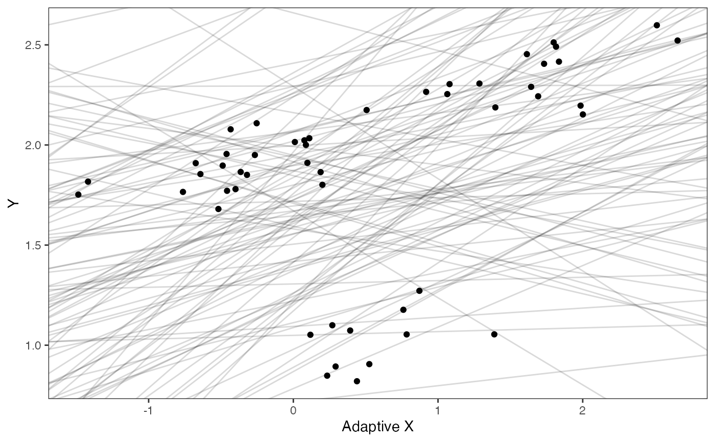

We will use the helper function blouch.reg.adapt.prep() to setup the dat file for Stan. Here “Z_adapt” is the number of predictors, and “regimes” is the name of the regime column in trdata$dat.

dat<-blouch.reg.adapt.prep(trdata,"Y_with_error","Y_error","X_with_error","X_error",Z_adaptive=1,"regimes",hl.prior,vy.prior,optima.prior,beta.prior)

Now we run the basic Multi-optima Adaptive Model, look at the results, and rstan::extract the posterior

fit.reg.adapt<- rstan::sampling(object = blouch:::stanmodels$blouchOU_reg_adapt,data = dat,chains = 2,cores = 2, iter =2000)
#> Found more than one class "stanfit" in cache; using the first, from namespace 'rstan'
#> Also defined by 'rethinking'
#> Found more than one class "stanfit" in cache; using the first, from namespace 'rstan'
#> Also defined by 'rethinking'

print(fit.reg.adapt,pars = c("hl","vy","optima","beta","beta_e"))
#> Inference for Stan model: blouchOU_reg_adapt.
#> 2 chains, each with iter=2000; warmup=1000; thin=1; 
#> post-warmup draws per chain=1000, total post-warmup draws=2000.
#> 
#>           mean se_mean   sd 2.5%  25%  50%  75% 97.5% n_eff Rhat
#> hl        0.23       0 0.12 0.07 0.15 0.20 0.28  0.51   872    1
#> vy        0.02       0 0.01 0.01 0.01 0.02 0.02  0.04  1237    1
#> optima[1] 2.03       0 0.06 1.92 1.99 2.02 2.06  2.14  2544    1
#> optima[2] 0.85       0 0.14 0.48 0.80 0.88 0.94  1.03  1011    1
#> beta[1]   0.24       0 0.05 0.16 0.21 0.23 0.27  0.38  1428    1
#> beta_e[1] 0.17       0 0.03 0.10 0.15 0.17 0.19  0.23  2776    1
#> 
#> Samples were drawn using NUTS(diag_e) at Tue Oct  8 13:49:43 2024.
#> For each parameter, n_eff is a crude measure of effective sample size,
#> and Rhat is the potential scale reduction factor on split chains (at 
#> convergence, Rhat=1).
post<-rstan::extract(fit.reg.adapt) #rstan::extract Posterior Distribution

Now lets look at the prior vs. posterior plots for the parameters Half-life plot

hl.post<-data.frame(post$hl)
names(hl.post)<-"post.hl.sims"

hl.plot<-ggplot2::ggplot()+
  ggplot2::geom_density(ggplot2::aes(prior.hl.sims,fill="prior.hl.sims"),alpha=0.2,data=hl.sims)+
  ggplot2::geom_density(ggplot2::aes(post.hl.sims,fill="post.hl.sims"),alpha=0.2,data=hl.post)+
  ggplot2::theme_bw()+
  ggplot2::theme(
    panel.grid.major = ggplot2::element_blank(),
    panel.grid.minor = ggplot2::element_blank())+
  
  #labs(title="Prior vs. Posterior Distribution ",x="Half-life", y = "Density")+
  ggplot2::labs(title="",x="Half-life", y = "Density")+
  
  #scale_fill_manual(labels=c("Posterior","Prior"))+
  ggplot2::geom_vline(xintercept=c(hl),linetype=2)+
  ggsci::scale_fill_npg(name="",labels=c("Posterior","Prior"))

hl.plot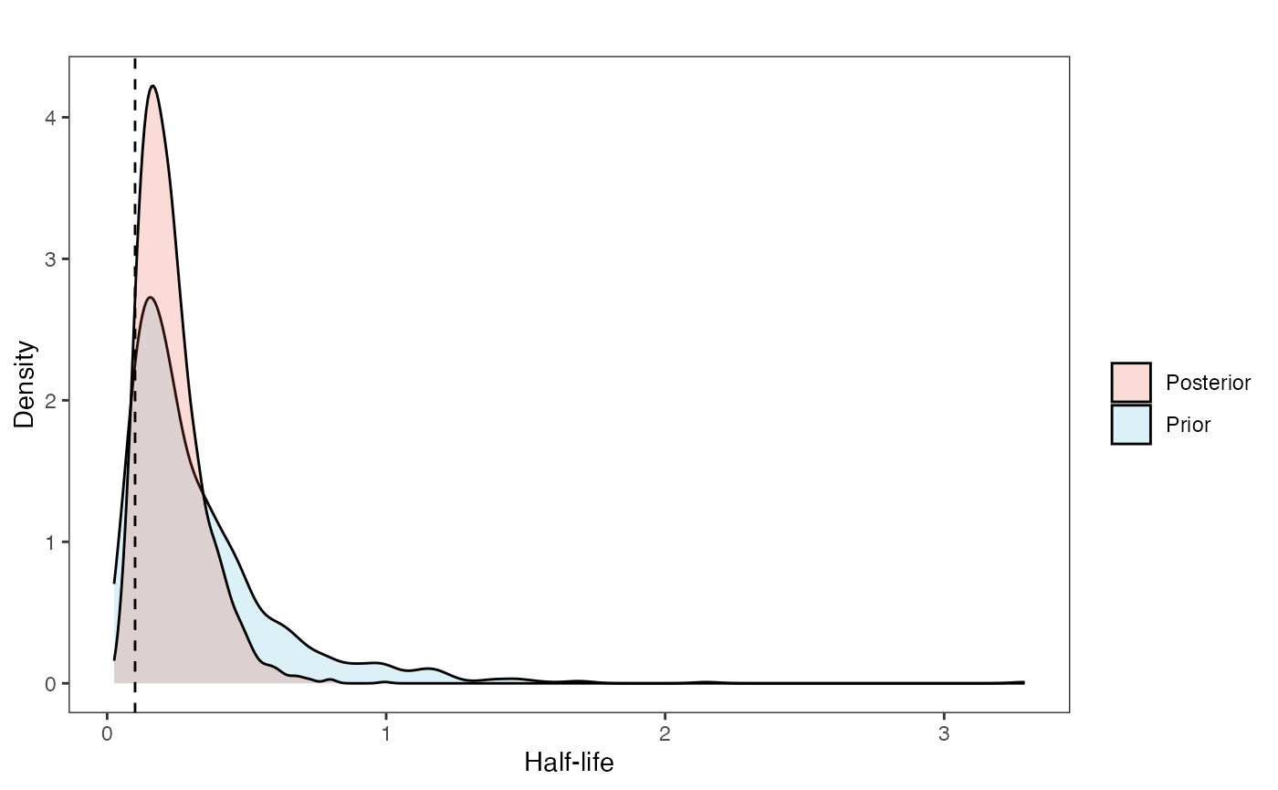

Vy Prior vs. posterior plot

vy.post<-data.frame(post$vy)
names(vy.post)<-"post.vy.sims"


vy.plot<-ggplot2::ggplot()+
  ggplot2::geom_density(ggplot2::aes(prior.vy.sims,fill="prior.vy.sims"),alpha=0.2,data=vy.sims)+
  ggplot2::geom_density(ggplot2::aes(post.vy.sims,fill="post.vy.sims"),alpha=0.2,data=vy.post)+
  ggplot2::theme_bw()+
  ggplot2::theme(
    panel.grid.major = ggplot2::element_blank(),
    panel.grid.minor = ggplot2::element_blank())+
  
  #labs(title="Prior vs. Posterior Distribution ",x="vy", y = "Density")+
  ggplot2::labs(title="",x="vy", y = "Density")+
  ggplot2::geom_vline(xintercept=c(vy),linetype=2)+
  
  #scale_fill_manual(labels=c("Posterior","Prior"))+
  ggsci::scale_fill_npg(name="",labels=c("Posterior","Prior"))

vy.plot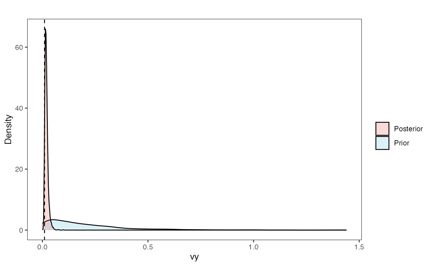

Prior versus posterior on how shared branch lengths correspond to covariance

a.sims<-log(2)/hl.sims;
sigma2_y.sims<-vy.sims*(2*(log(2)/hl.sims));
#x<-seq(from=0,to=1,by=0.001)
#V.sim<-calc_direct_V(phy,a.sims,sigma2_y.sims)


plot( NULL , xlim=c(0,1) , ylim=c(0,0.4) , xlab="Time since MRCA" , ylab="Covariance" ,cex.axis=0.75, mgp=c(1.25,0.25,0),tcl=-0.25)
for (i in 1:30){
  curve(calc_adaptive_cov_plot(a.sims[i,],sigma2_y.sims[i,],beta[3],x) , add=TRUE , lwd=4 , col=rethinking::col.alpha(1,0.15))
}

for (i in 1:30){
  curve(calc_adaptive_cov_plot(post$a[i],post$sigma2_y[i],post$beta[i],x) , add=TRUE , lwd=4 , col=rethinking::col.alpha(2,0.5))
}

#multiple traits


par(mar=c(3,3,0.25,0.25))

Prior vs. Posterior Plot for Regression

optima.sims<-rnorm(100,optima.prior[1],optima.prior[2])
beta.sims<-rnorm(n=100,beta.prior[1],beta.prior[2])

optima.post<-post$optima
beta.post<-data.frame(post$beta)
names(beta.post)<-c("post.beta.1")

mu.link.11<-function(x.seq){optima.post[,1]+x.seq*beta.post[,1]}
mu.link.12<-function(x.seq){optima.post[,2]+x.seq*beta.post[,1]}

x.seq <- seq(from=min(X), to=max(X) , length.out=100)
mu.11 <- sapply(x.seq , mu.link.11 )
mu.12 <- sapply(x.seq , mu.link.12 )


mu.mean.11<-colMeans(mu.11)
mu.mean.12<-colMeans(mu.12)

mu.mean.11<-data.frame(as.numeric(mu.mean.11))
mu.mean.12<-data.frame(as.numeric(mu.mean.12))

names(mu.mean.11)<-"mu.mean.11"
names(mu.mean.12)<-"mu.mean.12"

mu.CI.11 <- apply( mu.11 , MARGIN=2, FUN=rethinking::PI , prob=0.89 )
mu.CI.12 <- apply( mu.12 , MARGIN=2, FUN=rethinking::PI , prob=0.89 )


mu.CI.11<-data.frame(t(data.frame(mu.CI.11)),x.seq)
mu.CI.12<-data.frame(t(data.frame(mu.CI.12)),x.seq)

names(mu.CI.11)<-c("min.5.5","max.94.5","x.seq")
names(mu.CI.12)<-c("min.5.5","max.94.5","x.seq")

#df<-data.frame(Y=stan_sim_data$Y,X=stan_sim_data$direct_cov)
df<-data.frame(Y=dat$Y_obs,X=dat$X_obs,Regimes=regimes_tip)
df11<-data.frame(x.seq,mu.mean.11)
df12<-data.frame(x.seq,mu.mean.12)

#slope.prior.plot<-ggplot(data=reg.trdata$dat,aes(y=Sim1,x=X))+
slope.plot.1<-ggplot2::ggplot()+  
  ggplot2::geom_point(data=df,ggplot2::aes(y=Y,x=X,color=as.factor(Regimes)))+
  ggplot2::geom_abline(intercept=optima.sims,slope=beta.sims,alpha=0.05)+ #Prior
  ggplot2::geom_abline(intercept=beta[1],slope=beta[3],alpha=0.5,linetype=2)+
  ggplot2::geom_abline(intercept=beta[2],slope=beta[3],alpha=0.5,linetype=2)+
  ggplot2::geom_ribbon(data=mu.CI.11,ggplot2::aes(x=x.seq,ymin=min.5.5,ymax=max.94.5),linetype=2,alpha=0.1)+
  ggplot2::geom_line(data=df11,ggplot2::aes(x=x.seq,y=mu.mean.11),linetype=1,linewidth=1,alpha=0.3)+
  ggplot2::geom_ribbon(data=mu.CI.12,ggplot2::aes(x=x.seq,ymin=min.5.5,ymax=max.94.5),linetype=2,alpha=0.1)+
  ggplot2::geom_line(data=df12,ggplot2::aes(x=x.seq,y=mu.mean.12),linetype=1,linewidth=1,alpha=0.3)+
  ggplot2::theme_bw()+
  ggplot2::theme(
    panel.grid.major = ggplot2::element_blank(),
    panel.grid.minor = ggplot2::element_blank())+
  
  #ggtitle("Prior vs. Posterior for Intercept and Slope")+
  ggplot2::ylab("Y") + ggplot2::xlab("Direct Effect X")+ggplot2::labs(color="Regimes")+
  ggsci::scale_color_npg()

slope.plot.1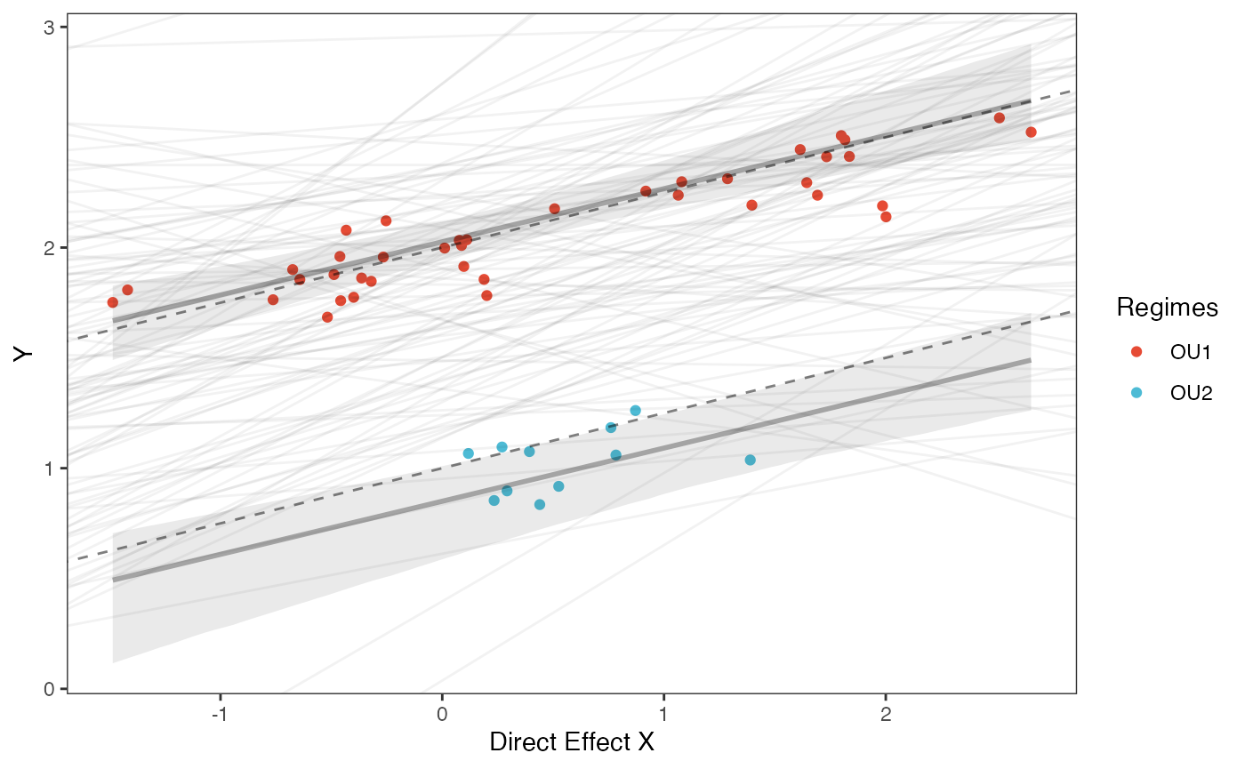

#Label points

Here is the Multilevel version of the same model Next we will set the priors for the estimated parameters - for this model this includes the half-life, Vy, optima, and beta. For the latter two parameters we will use the results of the linear model to inform our priors.

############################################################################################################
#Set Priors
hl.prior<-c(log(0.25),0.25)
vy.prior<-5
optima.prior<-c(1.5,0.5) #Informed by linear model
beta.prior<-c(0,0.25) #Informed by linear model
sigma.prior<-c(0,1)

############################################################################################################
#Make trdata file
trdata$dat<-cbind(trdata$dat,data.frame(cbind(Y_with_error,Y_error,X_with_error,X_error)))
############################################################################################################
dat<-blouch.reg.adapt.mlm.prep(trdata,"Y_with_error","Y_error","X_with_error","X_error",Z_adaptive=1,"regimes",hl.prior,vy.prior,optima.prior,beta.prior,sigma.prior)

fit.reg.adapt.mlm.vi<- rstan::sampling(object = blouch:::stanmodels$blouchOU_reg_adapt_mlm_vi,data = dat,chains = 2,cores=2,iter =2000)
#> Found more than one class "stanfit" in cache; using the first, from namespace 'rstan'
#> Also defined by 'rethinking'
#> Found more than one class "stanfit" in cache; using the first, from namespace 'rstan'
#> Also defined by 'rethinking'

print(fit.reg.adapt.mlm.vi,pars = c("hl","vy","optima","beta","beta_e","sigma"))
#> Inference for Stan model: blouchOU_reg_adapt_mlm_vi.
#> 2 chains, each with iter=2000; warmup=1000; thin=1; 
#> post-warmup draws per chain=1000, total post-warmup draws=2000.
#> 
#>           mean se_mean   sd 2.5%  25%  50%  75% 97.5% n_eff Rhat
#> hl        0.25    0.00 0.06 0.15 0.21 0.24 0.28  0.39  1880    1
#> vy        0.02    0.00 0.01 0.01 0.02 0.02 0.02  0.03  2482    1
#> optima[1] 2.04    0.00 0.06 1.91 2.00 2.04 2.07  2.16  3475    1
#> optima[2] 0.84    0.00 0.11 0.58 0.77 0.85 0.91  1.03  2165    1
#> beta[1]   0.23    0.00 0.05 0.14 0.20 0.24 0.27  0.34  3130    1
#> beta_e[1] 0.16    0.00 0.03 0.09 0.14 0.16 0.18  0.22  3536    1
#> sigma     0.92    0.01 0.43 0.34 0.59 0.83 1.15  2.00  2906    1
#> 
#> Samples were drawn using NUTS(diag_e) at Tue Oct  8 13:50:15 2024.
#> For each parameter, n_eff is a crude measure of effective sample size,
#> and Rhat is the potential scale reduction factor on split chains (at 
#> convergence, Rhat=1).
post<-rstan::extract(fit.reg.adapt.mlm.vi)

And the non-centered version

fit.reg.adapt.mlm.vi.nc<- rstan::sampling(object = blouch:::stanmodels$blouchOU_reg_adapt_mlm_vi_nc,data = dat,chains = 2,cores=2,iter =2000)
#> Found more than one class "stanfit" in cache; using the first, from namespace 'rstan'
#> Also defined by 'rethinking'
#> Found more than one class "stanfit" in cache; using the first, from namespace 'rstan'
#> Also defined by 'rethinking'
#> Warning: There were 15 divergent transitions after warmup. See
#> https://mc-stan.org/misc/warnings.html#divergent-transitions-after-warmup
#> to find out why this is a problem and how to eliminate them.
#> Warning: Examine the pairs() plot to diagnose sampling problems

print(fit.reg.adapt.mlm.vi.nc,pars = c("hl","vy","optima","beta","beta_e","sigma"))
#> Inference for Stan model: blouchOU_reg_adapt_mlm_vi_nc.
#> 2 chains, each with iter=2000; warmup=1000; thin=1; 
#> post-warmup draws per chain=1000, total post-warmup draws=2000.
#> 
#>           mean se_mean   sd 2.5%  25%  50%  75% 97.5% n_eff Rhat
#> hl        0.25    0.00 0.06 0.15 0.21 0.24 0.28  0.38  1849    1
#> vy        0.02    0.00 0.01 0.01 0.02 0.02 0.02  0.03  2024    1
#> optima[1] 2.04    0.00 0.06 1.92 2.00 2.03 2.07  2.16  2378    1
#> optima[2] 0.84    0.00 0.11 0.59 0.77 0.85 0.92  1.03  1822    1
#> beta[1]   0.23    0.00 0.05 0.14 0.20 0.23 0.26  0.33  2439    1
#> beta_e[1] 0.16    0.00 0.03 0.09 0.14 0.16 0.18  0.21  2610    1
#> sigma     0.90    0.01 0.40 0.37 0.60 0.82 1.12  1.86  1098    1
#> 
#> Samples were drawn using NUTS(diag_e) at Tue Oct  8 13:51:44 2024.
#> For each parameter, n_eff is a crude measure of effective sample size,
#> and Rhat is the potential scale reduction factor on split chains (at 
#> convergence, Rhat=1).
post<-rstan::extract(fit.reg.adapt.mlm.vi.nc)

From there the posteriors should be explored, compared to the priors, etc. See the Simulation Example for one example of how to do this.

rm(list=ls())

Multi-optima Direct Effect and Adaptive Model

We will now include both regimes painted on the tree and a direct effect and adaptive predictor

############################################################################################################
#Regimes + Adaptive + Direct Model
############################################################################################################
#Create phylogeny
########################################################################################################
N<-50 #Number of species
set.seed(10) #Set seed to get same random species each time

phy <- ape::keep.tip(tree.10K,sample(tree.10K$tip.label)[1:N]) 
phy<-ape::multi2di(phy)

l.tree<-max(ape::branching.times(phy)) ## rescale tree to height 1
phy$edge.length<-phy$edge.length/l.tree 

tip.label<-phy$tip.label

#Set regimes - manually - 2 regimes
#Locate nodes
plot(phy,no.margin=TRUE,edge.width=2,cex=0.7)
ape::nodelabels(frame="none",adj=c(1.1,-0.4))
ape::tiplabels()

#Paint Regimes on Tree
shifts<-c(84) #Location of nodes with regime shifts
trdata<-data.frame(phy$tip.label)
trdata<-treeplyr::make.treedata(phy,trdata)
trdata<-set.converge.regimes(trdata,shifts)
#> [1] 1
#>  [1] OU1 OU1 OU1 OU1 OU1 OU1 OU1 OU1 OU1 OU1 OU1 OU1 OU1 OU1 OU1 OU1 OU1 OU1 OU1
#> [20] OU1 OU1 OU1 OU1 OU1 OU1 OU1 OU1 OU1 OU1 OU1 OU1 OU1 OU1 OU1 OU1 OU1 OU1 OU1
#> [39] OU1 OU1 OU1 OU1 OU1 OU1 OU1 OU1 OU1 OU1 OU1 OU1 OU1 OU1 OU1 OU1 OU1 OU1 OU1
#> [58] OU1 OU1 OU1 OU1 OU1 OU1 OU1 OU2 OU2 OU2 OU2 OU2 OU2 OU2 OU2 OU2 OU2 OU2 OU2
#> [77] OU2 OU2 OU2 OU2 OU2 OU2 OU2 OU2 OU2 OU1 OU1 OU1 OU1 OU1 OU1 OU1 OU1 OU1 OU1
#> [96] OU1 OU1 OU1
#> Levels: OU1 OU2
#> [1] "#E64B35FF" "#4DBBD5FF"

#Check if manual setting code worked
shifts.total<-c(trdata$dat$regimes,trdata$phy$node.label)
edge.regimes <- factor(shifts.total[trdata$phy$edge[,2]])
print(edge.regimes)
#>  [1] OU1 OU1 OU1 OU1 OU1 OU1 OU1 OU1 OU1 OU1 OU1 OU1 OU1 OU1 OU1 OU1 OU1 OU1 OU1
#> [20] OU1 OU1 OU1 OU1 OU1 OU1 OU1 OU1 OU1 OU1 OU1 OU1 OU1 OU1 OU1 OU1 OU1 OU1 OU1
#> [39] OU1 OU1 OU1 OU1 OU1 OU1 OU1 OU1 OU1 OU1 OU1 OU1 OU1 OU1 OU1 OU1 OU1 OU1 OU1
#> [58] OU1 OU1 OU1 OU1 OU1 OU1 OU1 OU2 OU2 OU2 OU2 OU2 OU2 OU2 OU2 OU2 OU2 OU2 OU2
#> [77] OU2 OU2 OU2 OU2 OU2 OU2 OU2 OU2 OU2 OU1 OU1 OU1 OU1 OU1 OU1 OU1 OU1 OU1 OU1
#> [96] OU1 OU1 OU1
#> Levels: OU1 OU2

reg.colors <- ggsci::pal_aaas("default", alpha = 0.7)(2)
print(reg.colors)
#> [1] "#3B4992B2" "#EE0000B2"
plot(trdata$phy,edge.color = reg.colors[edge.regimes], edge.width = 1, cex = 0.2)

#Phylogeny info
n<-length(trdata$phy$tip.label)

regimes_internal <-trdata$phy$node.label
regimes_tip <- trdata$dat$regimes
regimes <- concat.factor(regimes_tip, regimes_internal)
anc_maps<-"regimes"
lineages <- lapply(1:n, function(e) lineage.constructor(trdata$phy, e, anc_maps, regimes)) #Trace lineage from tips (n) to root and determine regimes of each node or branch

############################################################################################################
hl<-0.1 #0.1, 0.25, 0.75 - testing options
a<-log(2)/hl
vy<-0.01 #0.25,0.5 - testing options
sigma2_y<-vy*(2*(log(2)/hl));

vX0<-0
vY0 <- 0

Z_direct<-1
Z_adaptive<-1
Z<-Z_direct+Z_adaptive
sigma2_x<-matrix(1,1,1) #Variance of BM Process

Xd<-rnorm(N,0,1)
names(Xd)<-phy$tip.label
phytools::phenogram(phy,Xd,spread.labels=TRUE,spread.cost=c(1,0)) #Plot X data
#> Optimizing the positions of the tip labels...

Xa<-phytools::fastBM(phy,a=vX0,sig2=sigma2_x[1,1],internal=FALSE) #Simulate X BM variable on tree, with scaling 10
phytools::phenogram(phy,Xa,spread.labels=TRUE,spread.cost=c(1,0)) #Plot X data
#> Optimizing the positions of the tip labels...

#sigma2_x<-ratematrix(phy,Xa) #Calculate evolutionary v/cv matrix
Xs<-cbind(Xd,Xa)

dmX<-weight.matrix(trdata$phy, a, lineages) #Slouch approach
dmX<-cbind(dmX,calc_mixed_dmX(phy,a,Xs,Z_direct,Z_adaptive))

beta<-c(2,1,0.35,0.25) #Two Optima/Two Slopes
mu<-dmX%*%beta #Simulate mu for Y

V<-calc_adaptive_V(phy,a, sigma2_y,   beta[length(beta)],  sigma2_x,Z_adaptive)
Y<-MASS::mvrnorm(n=1,mu,V)

################################################################################################################
#Plot data
df<-data.frame(Y=Y,Xd=Xs[,1],Xa=Xs[,2])

ggplot2::ggplot(data=df,ggplot2::aes(x=Xd,y=Y))+
  ggplot2::geom_point()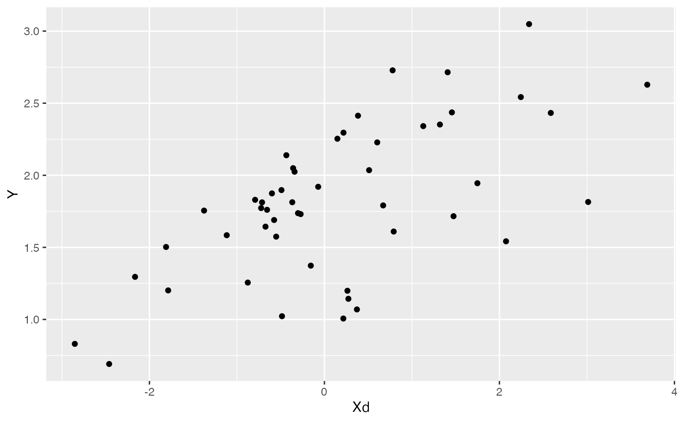

ggplot2::ggplot(data=df,ggplot2::aes(x=Xa,y=Y))+
  ggplot2::geom_point()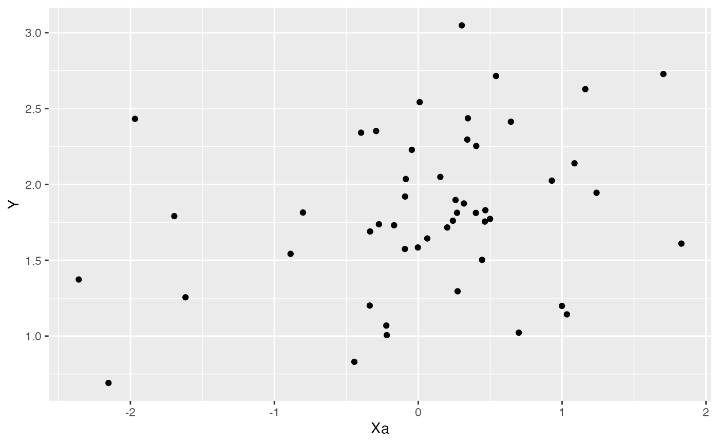

summary(lm(Y~Xs,df))
#> 
#> Call:
#> lm(formula = Y ~ Xs, data = df)
#> 
#> Residuals:
#>      Min       1Q   Median       3Q      Max 
#> -0.84900 -0.16208  0.08845  0.25892  0.67924 
#> 
#> Coefficients:
#>             Estimate Std. Error t value Pr(>|t|)    
#> (Intercept)  1.78206    0.05601  31.818  < 2e-16 ***
#> XsXd         0.23270    0.04105   5.668 8.52e-07 ***
#> XsXa         0.14175    0.06396   2.216   0.0315 *  
#> ---
#> Signif. codes:  0 '***' 0.001 '**' 0.01 '*' 0.05 '.' 0.1 ' ' 1
#> 
#> Residual standard error: 0.3935 on 47 degrees of freedom
#> Multiple R-squared:  0.4563, Adjusted R-squared:  0.4332 
#> F-statistic: 19.72 on 2 and 47 DF,  p-value: 6.034e-07

########################################################################################################
#Simulate errors - for use with blouchOU_reg_direct_adaptive_ME
Z_X_error<-2 #Number of X traits with error
X_error<-matrix(0.01,nrow=N,ncol=Z_X_error)
X_error<-data.frame(X_error)
names(X_error)<-c("Xd_error","Xa_error")
Y_error<-rep(0.01,N)
Y_with_error<-Y+rnorm(N,0,0.01)
X_with_error<-apply(Xs,2,function(X){X+rnorm(N,0,0.01)})

############################################################################################################
#Set Priors
hl.prior<-c(log(0.25),0.25)
vy.prior<-5
optima.prior<-c(1.5,0.5) #Informed by linear model
beta.prior<-c(0,0.25) #Informed by linear model

Half-life Prior plot

hl.sims<-data.frame(rlnorm(n=1000,meanlog=hl.prior[1],sdlog=hl.prior[2]))
names(hl.sims)<-"prior.hl.sims"

hl.prior.plot<-ggplot2::ggplot()+
  ggplot2::geom_density(ggplot2::aes(prior.hl.sims,fill="prior.hl.sims"),alpha=0.2,data=hl.sims)+
  ggplot2::theme_bw()+
  ggplot2::theme(
    panel.grid.major = ggplot2::element_blank(),
    panel.grid.minor = ggplot2::element_blank())+
  
  #labs(title="Prior vs. Posterior Distribution ",x="Half-life", y = "Density")+
  ggplot2::labs(title="",x="Half-life", y = "Density")+
  
  #scale_fill_manual(labels=c("Posterior","Prior"))+
  ggplot2::geom_vline(xintercept=c(hl),linetype=2)+
  ggsci::scale_fill_npg(name="",labels=c("Prior"))

hl.prior.plot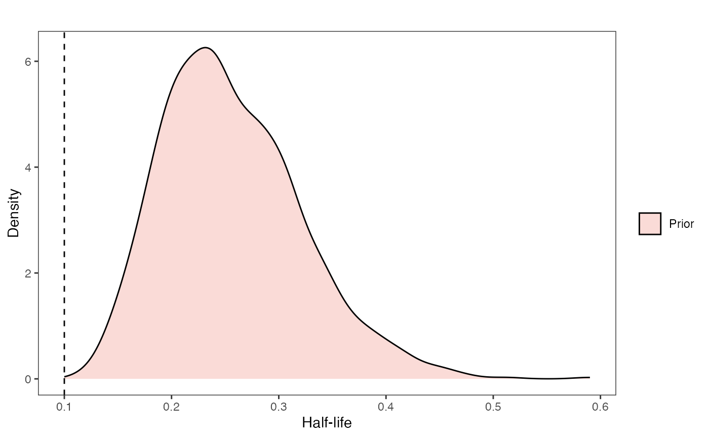

Vy Prior Plot

vy.sims<-rexp(n=1000,rate=vy.prior)
vy.sims<-data.frame(vy.sims)
names(vy.sims)<-"prior.vy.sims"

vy.prior.plot<-ggplot2::ggplot()+
  ggplot2::geom_density(ggplot2::aes(prior.vy.sims,fill="prior.vy.sims"),alpha=0.2,data=vy.sims)+
  ggplot2::theme_bw()+
  ggplot2::theme(
    panel.grid.major = ggplot2::element_blank(),
    panel.grid.minor = ggplot2::element_blank())+
  
  #labs(title="Prior vs. Posterior Distribution ",x="vy", y = "Density")+
  ggplot2::labs(title="",x="vy", y = "Density")+
  ggplot2::geom_vline(xintercept=c(vy),linetype=2)+
  
  #scale_fill_manual(labels=c("Posterior","Prior"))+
  ggsci::scale_fill_npg(name="",labels=c("Prior"))


vy.prior.plot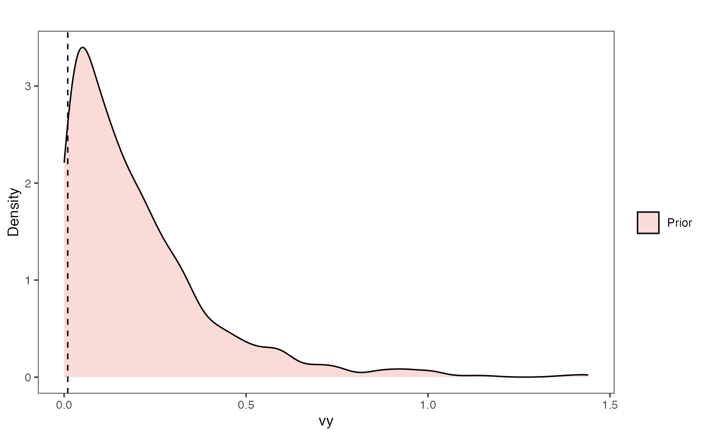

Adaptation model

a.sims<-log(2)/hl.sims;
sigma2_y.sims<-vy.sims*(2*(log(2)/hl.sims));
#x<-seq(from=0,to=1,by=0.001)
#V.sim<-calc_direct_V(phy,a.sims,sigma2_y.sims)


plot( NULL , xlim=c(0,1) , ylim=c(0,0.4) , xlab="Time since MRCA" , ylab="Covariance" ,cex.axis=0.75, mgp=c(1.25,0.25,0),tcl=-0.25)
for (i in 1:30){
  curve(calc_adaptive_cov_plot(a.sims[i,],sigma2_y.sims[i,],beta[3],x) , add=TRUE , lwd=4 , col=rethinking::col.alpha(1,0.15))
}

par(mar=c(3,3,0.25,0.25))
covariance.plot <- recordPlot()
dev.off()
#> null device 
#>           1

covariance.plot

Prior vs. Posterior Plot

optima.sims<-rnorm(100,optima.prior[1],optima.prior[2])
beta.sims<-rnorm(n=100,beta.prior[1],beta.prior[2])

df<-data.frame(Y=Y_with_error,X=X_with_error,Regimes=regimes_tip)

slope.plot.Xd<-ggplot2::ggplot()+  
  ggplot2::geom_point(data=df,ggplot2::aes(y=Y,x=X.Xd,color=Regimes))+
  ggplot2::geom_abline(intercept=optima.sims,slope=beta.sims,alpha=0.15)+ #Prior
  ggplot2::theme_bw()+
  ggplot2::theme(
  panel.grid.major = ggplot2::element_blank(),
  panel.grid.minor = ggplot2::element_blank())+
  ggplot2::ylab("Y") + ggplot2::xlab("Direct effect trait")+
  ggsci::scale_color_npg()

slope.plot.Xd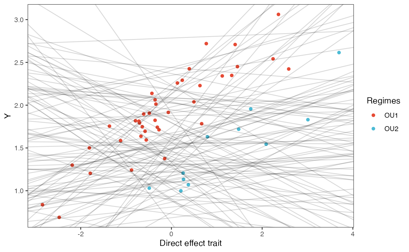

slope.plot.Xa<-ggplot2::ggplot()+  
  ggplot2::geom_point(data=df,ggplot2::aes(y=Y,x=X.Xa,color=Regimes))+
  ggplot2::geom_abline(intercept=optima.sims,slope=beta.sims,alpha=0.15)+ #Prior
  ggplot2::theme_bw()+
  ggplot2::theme(
  panel.grid.major = ggplot2::element_blank(),
  panel.grid.minor = ggplot2::element_blank())+
  ggplot2::ylab("Y") + ggplot2::xlab("Adaptive trait")+
  ggsci::scale_color_npg()

slope.plot.Xa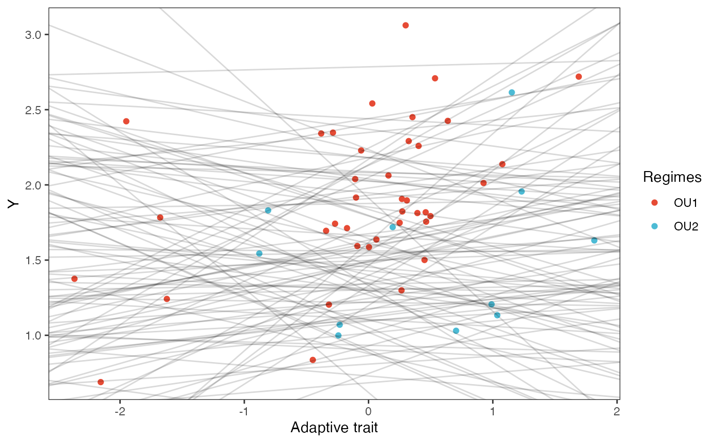

############################################################################################################
#Make trdata file
trdata$dat<-cbind(trdata$dat,data.frame(cbind(Y_with_error,Y_error,X_with_error,X_error)))

We will use the helper function blouch.reg.direct.adapt.prep() to setup the dat file for Stan. Here the names of the direct effect and adaptive columns are “Xd”, and “Xa” and their associated errors, with Z_direct and Z_adaptive th number of direct and adaptive traits, respectively, and “regimes” is the name of the regimes column data in trdata$dat.

############################################################################################################
dat<-blouch.reg.direct.adapt.prep(trdata,"Y_with_error","Y_error",c("Xd","Xa"),c("Xd_error","Xa_error"),Z_direct=1,Z_adaptive=1,"regimes",hl.prior,vy.prior,optima.prior,beta.prior)

First we run the basic Multi-optima Direct Effect Adaptive Model.

fit.reg.direct.adapt<- rstan::sampling(object = blouch:::stanmodels$blouchOU_reg_direct_adapt,data = dat,chains = 2,cores=2,iter =2000)
#> Found more than one class "stanfit" in cache; using the first, from namespace 'rstan'
#> Also defined by 'rethinking'
#> Found more than one class "stanfit" in cache; using the first, from namespace 'rstan'
#> Also defined by 'rethinking'

print(fit.reg.direct.adapt,pars = c("hl","vy","optima","beta","beta_e"))
#> Inference for Stan model: blouchOU_reg_direct_adapt.
#> 2 chains, each with iter=2000; warmup=1000; thin=1; 
#> post-warmup draws per chain=1000, total post-warmup draws=2000.
#> 
#>           mean se_mean   sd 2.5%  25%  50%  75% 97.5% n_eff Rhat
#> hl        0.21       0 0.05 0.13 0.18 0.21 0.25  0.33  1792    1
#> vy        0.01       0 0.00 0.00 0.01 0.01 0.01  0.02  2638    1
#> optima[1] 1.98       0 0.05 1.88 1.95 1.98 2.01  2.09  4501    1
#> optima[2] 0.95       0 0.09 0.77 0.89 0.95 1.01  1.11  2045    1
#> beta[1]   0.35       0 0.01 0.33 0.34 0.35 0.35  0.36  3624    1
#> beta[2]   0.33       0 0.05 0.25 0.30 0.33 0.36  0.44  1504    1
#> beta_e[1] 0.23       0 0.03 0.18 0.21 0.23 0.25  0.29  2259    1
#> 
#> Samples were drawn using NUTS(diag_e) at Tue Oct  8 13:52:17 2024.
#> For each parameter, n_eff is a crude measure of effective sample size,
#> and Rhat is the potential scale reduction factor on split chains (at 
#> convergence, Rhat=1).
post<-rstan::extract(fit.reg.direct.adapt) #rstan::extract posterior

Prior vs. posterior

hl.sims<-data.frame(rlnorm(n=1000,meanlog=hl.prior[1],sdlog=hl.prior[2]))
names(hl.sims)<-"prior.hl.sims"

hl.post<-data.frame(post$hl)
names(hl.post)<-"post.hl.sims"

hl.plot<-ggplot2::ggplot()+
  ggplot2::geom_density(ggplot2::aes(prior.hl.sims,fill="prior.hl.sims"),alpha=0.2,data=hl.sims)+
  ggplot2::geom_density(ggplot2::aes(post.hl.sims,fill="post.hl.sims"),alpha=0.2,data=hl.post)+
  ggplot2::theme_bw()+
  ggplot2::theme(
  panel.grid.major = ggplot2::element_blank(),
  panel.grid.minor = ggplot2::element_blank())+
  ggplot2::labs(title="",x="Half-life", y = "Density")+
  ggplot2::geom_vline(xintercept=c(hl),linetype=2)+
  ggsci::scale_fill_npg(name="",labels=c("Posterior","Prior"))

hl.plot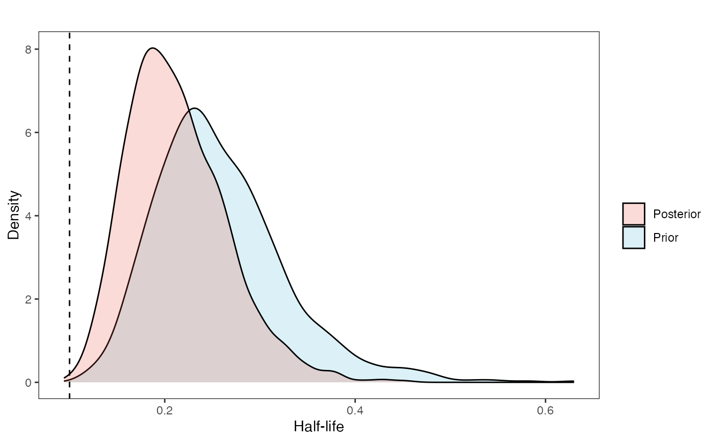

Prior vs. posterior plot

vy.sims<-rexp(n=1000,rate=vy.prior)
vy.sims<-data.frame(vy.sims)
names(vy.sims)<-"prior.vy.sims"

vy.post<-data.frame(post$vy)
names(vy.post)<-"post.vy.sims"


vy.plot<-ggplot2::ggplot()+
  ggplot2::geom_density(ggplot2::aes(prior.vy.sims,fill="prior.vy.sims"),alpha=0.2,data=vy.sims)+
  ggplot2::geom_density(ggplot2::aes(post.vy.sims,fill="post.vy.sims"),alpha=0.2,data=vy.post)+
  ggplot2::theme_bw()+
  ggplot2::theme(
  panel.grid.major = ggplot2::element_blank(),
  panel.grid.minor = ggplot2::element_blank())+
  ggplot2::labs(title="",x="vy", y = "Density")+
  ggplot2::geom_vline(xintercept=c(vy),linetype=2)+
  ggsci::scale_fill_npg(name="",labels=c("Posterior","Prior"))

vy.plot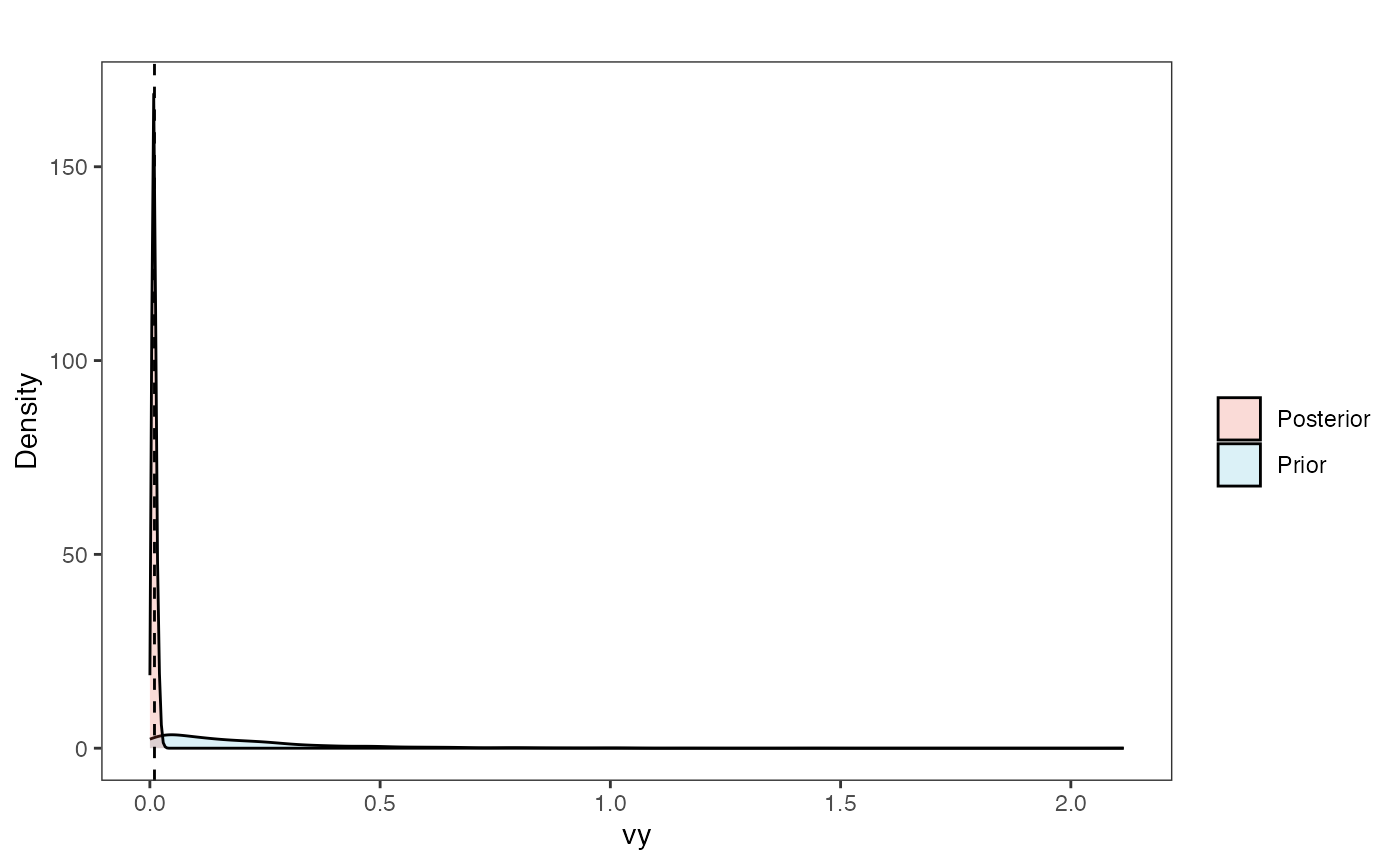

Adaptation model

a.sims<-log(2)/hl.sims;
sigma2_y.sims<-vy.sims*(2*(log(2)/hl.sims));
#x<-seq(from=0,to=1,by=0.001)
#V.sim<-calc_direct_V(phy,a.sims,sigma2_y.sims)


plot( NULL , xlim=c(0,1) , ylim=c(0,0.4) , xlab="Time since MRCA" , ylab="Covariance" ,cex.axis=0.75, mgp=c(1.25,0.25,0),tcl=-0.25)
for (i in 1:30){
  curve(calc_adaptive_cov_plot(a.sims[i,],sigma2_y.sims[i,],beta[3:4],x) , add=TRUE , lwd=4 , col=rethinking::col.alpha(1,0.15))
}

for (i in 1:30){
  curve(calc_adaptive_cov_plot(post$a[i],post$sigma2_y[i],post$beta[i,],x) , add=TRUE , lwd=4 , col=rethinking::col.alpha(2,0.5))
}

#multiple traits


par(mar=c(3,3,0.25,0.25))
covariance.plot <- recordPlot()
dev.off()
#> null device 
#>           1

#Vt = sigma2_y /( 2 * a) * ((1 - exp(-2 * a * ta)) .* exp(-a * tij)); //From Hansen (1997)

covariance.plot

Slope plots for direct and adaptive models with Measurement Error

library(ggsci)

optima.sims<-rnorm(100,optima.prior[1],optima.prior[2])
beta.sims<-rnorm(n=100,beta.prior[1],beta.prior[2])

optima.post<-post$optima

beta.post.1<-data.frame(post$beta[,1])
names(beta.post.1)<-"post.beta.1"

beta.post.2<-data.frame(post$beta[,2])
names(beta.post.2)<-"post.beta.2"

mu.link.11<-function(x.seq){optima.post[,1]+x.seq*beta.post.1}
mu.link.12<-function(x.seq){optima.post[,2]+x.seq*beta.post.1}
mu.link.21<-function(x.seq){optima.post[,1]+x.seq*beta.post.2}
mu.link.22<-function(x.seq){optima.post[,2]+x.seq*beta.post.2}
x.seq <- seq(from=min(Xs), to=max(Xs) , length.out=100)
mu.11 <- sapply(x.seq , mu.link.11 )
mu.12 <- sapply(x.seq , mu.link.12 )
mu.21 <- sapply(x.seq , mu.link.21 )
mu.22 <- sapply(x.seq , mu.link.22 )
mu.mean.11 <-lapply( mu.11 , mean )
mu.mean.12 <-lapply( mu.12 , mean )
mu.mean.21 <-lapply( mu.21 , mean )
mu.mean.22 <-lapply( mu.22 , mean )

mu.mean.11<-data.frame(as.numeric(mu.mean.11))
mu.mean.12<-data.frame(as.numeric(mu.mean.12))
names(mu.mean.11)<-"mu.mean.11"
names(mu.mean.12)<-"mu.mean.12"
mu.mean.21<-data.frame(as.numeric(mu.mean.21))
mu.mean.22<-data.frame(as.numeric(mu.mean.22))
names(mu.mean.21)<-"mu.mean.21"
names(mu.mean.22)<-"mu.mean.22"

mu.CI.11 <- lapply( mu.11 , rethinking::PI , prob=0.89 )
mu.CI.12 <- lapply( mu.12 , rethinking::PI , prob=0.89 )
mu.CI.11<-data.frame(t(data.frame(mu.CI.11)),x.seq)
mu.CI.12<-data.frame(t(data.frame(mu.CI.12)),x.seq)

mu.CI.21 <- lapply( mu.21 , rethinking::PI , prob=0.89 )
mu.CI.22 <- lapply( mu.22 , rethinking::PI , prob=0.89 )
mu.CI.21<-data.frame(t(data.frame(mu.CI.21)),x.seq)
mu.CI.22<-data.frame(t(data.frame(mu.CI.22)),x.seq)

names(mu.CI.11)<-c("min.5.5","max.94.5","x.seq")
names(mu.CI.12)<-c("min.5.5","max.94.5","x.seq")
names(mu.CI.21)<-c("min.5.5","max.94.5","x.seq")
names(mu.CI.22)<-c("min.5.5","max.94.5","x.seq")

df<-data.frame(Y=dat$Y_obs,X=dat$X_obs,Regimes=regimes_tip)
df11<-data.frame(x.seq,mu.mean.11)
df12<-data.frame(x.seq,mu.mean.12)
df21<-data.frame(x.seq,mu.mean.21)
df22<-data.frame(x.seq,mu.mean.22)

slope.plot.Xd<-ggplot2::ggplot()+  
  ggplot2::geom_point(data=df,ggplot2::aes(y=Y,x=X.Xd,color=Regimes))+
  ggplot2::geom_abline(intercept=optima.sims,slope=beta.sims,alpha=0.15)+ #Prior
  ggplot2::geom_line(data=df11,ggplot2::aes(x=x.seq,y=mu.mean.11),linetype=1)+
  ggplot2::geom_abline(intercept=beta[1],slope=beta[3],alpha=0.5,linetype=2)+
  ggplot2::geom_abline(intercept=beta[2],slope=beta[3],alpha=0.5,linetype=2)+
  ggplot2::geom_ribbon(data=mu.CI.11,ggplot2::aes(x=x.seq,ymin=min.5.5,ymax=max.94.5),linetype=2,alpha=0.25)+
  ggplot2::geom_line(data=df12,ggplot2::aes(x=x.seq,y=mu.mean.12),linetype=1)+
  ggplot2::geom_ribbon(data=mu.CI.12,ggplot2::aes(x=x.seq,ymin=min.5.5,ymax=max.94.5),linetype=2,alpha=0.25)+
  ggplot2::theme_bw()+
  ggplot2::theme(
  panel.grid.major = ggplot2::element_blank(),
  panel.grid.minor = ggplot2::element_blank())+
  ggplot2::ylab("Y") + ggplot2::xlab("Direct effect trait")+
  ggsci::scale_color_npg()

slope.plot.Xd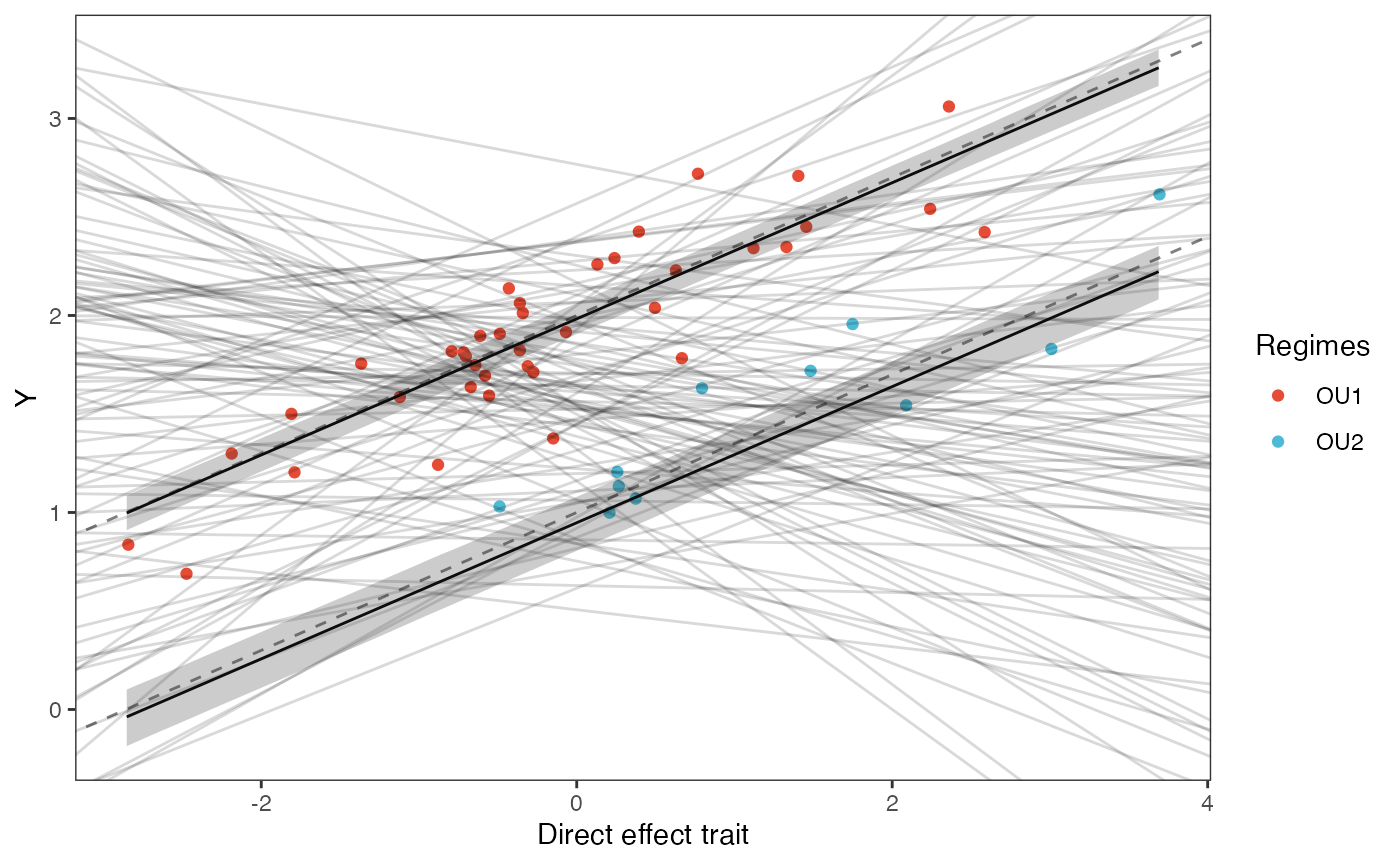

slope.plot.Xa<-ggplot2::ggplot()+  
  ggplot2::geom_point(data=df,ggplot2::aes(y=Y,x=X.Xa,color=Regimes))+
  ggplot2::geom_abline(intercept=optima.sims,slope=beta.sims,alpha=0.15)+ #Prior
  ggplot2::geom_abline(intercept=beta[1],slope=beta[4],alpha=0.5,linetype=2)+
  ggplot2::geom_abline(intercept=beta[2],slope=beta[4],alpha=0.5,linetype=2)+
  ggplot2::geom_line(data=df21,ggplot2::aes(x=x.seq,y=mu.mean.21),linetype=1)+
  ggplot2::geom_ribbon(data=mu.CI.21,ggplot2::aes(x=x.seq,ymin=min.5.5,ymax=max.94.5),linetype=2,alpha=0.25)+
  ggplot2::geom_line(data=df22,ggplot2::aes(x=x.seq,y=mu.mean.22),linetype=1)+
  ggplot2::geom_ribbon(data=mu.CI.22,ggplot2::aes(x=x.seq,ymin=min.5.5,ymax=max.94.5),linetype=2,alpha=0.25)+
  ggplot2::theme_bw()+
  ggplot2::theme(
  panel.grid.major = ggplot2::element_blank(),
  panel.grid.minor = ggplot2::element_blank())+
  ggplot2::ylab("Y") + ggplot2::xlab("Adaptive trait")+
  ggsci::scale_color_npg()

slope.plot.Xa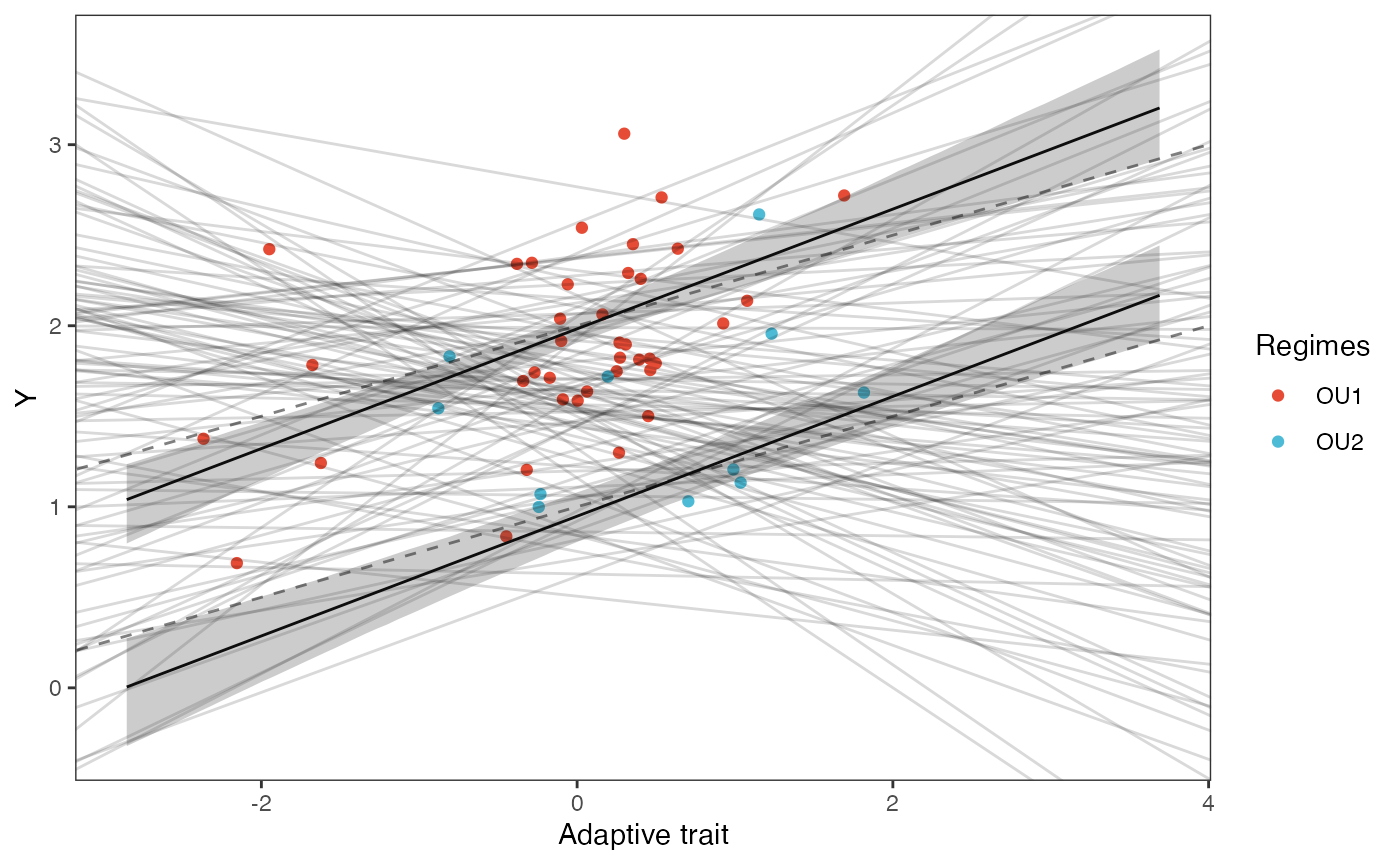

#Next we run the Multilevel version of the same model
############################################################################################################
#Set Priors
hl.prior<-c(log(0.25),0.25)
vy.prior<-5
optima.prior<-c(1.5,0.5) #Informed by linear model
beta.prior<-c(0,0.25) #Informed by linear model
sigma.prior<-c(0,1)

############################################################################################################
#Make trdata file
trdata$dat<-cbind(trdata$dat,data.frame(cbind(Y_with_error,Y_error,X_with_error,X_error)))

############################################################################################################
dat<-blouch.reg.direct.adapt.mlm.prep(trdata,"Y_with_error","Y_error",c("Xd","Xa"),c("Xd_error","Xa_error"),Z_direct=1,Z_adaptive=1,"regimes",hl.prior,vy.prior,optima.prior,beta.prior,sigma.prior)

Next we run the Multilevel version of the same model

fit.reg.direct.adapt.mlm.vi<- rstan::sampling(object = blouch:::stanmodels$blouchOU_reg_direct_adapt_mlm_vi,data = dat,chains = 2,cores=2,iter =2000)
#> Found more than one class "stanfit" in cache; using the first, from namespace 'rstan'
#> Also defined by 'rethinking'
#> Found more than one class "stanfit" in cache; using the first, from namespace 'rstan'
#> Also defined by 'rethinking'

print(fit.reg.direct.adapt.mlm.vi,pars = c("hl","vy","optima","beta","beta_e"))
#> Inference for Stan model: blouchOU_reg_direct_adapt_mlm_vi.
#> 2 chains, each with iter=2000; warmup=1000; thin=1; 
#> post-warmup draws per chain=1000, total post-warmup draws=2000.
#> 
#>           mean se_mean   sd 2.5%  25%  50%  75% 97.5% n_eff Rhat
#> hl        0.22       0 0.05 0.13 0.18 0.21 0.25  0.34  2022    1
#> vy        0.01       0 0.00 0.00 0.01 0.01 0.01  0.02  2938    1
#> optima[1] 1.98       0 0.05 1.89 1.95 1.98 2.02  2.08  3500    1
#> optima[2] 0.94       0 0.10 0.72 0.88 0.95 1.00  1.10  1848    1
#> beta[1]   0.35       0 0.01 0.33 0.34 0.35 0.35  0.36  4252    1
#> beta[2]   0.33       0 0.05 0.25 0.30 0.33 0.36  0.45  1886    1
#> beta_e[1] 0.23       0 0.03 0.18 0.22 0.23 0.25  0.29  2202    1
#> 
#> Samples were drawn using NUTS(diag_e) at Tue Oct  8 13:52:50 2024.
#> For each parameter, n_eff is a crude measure of effective sample size,
#> and Rhat is the potential scale reduction factor on split chains (at 
#> convergence, Rhat=1).
post<-rstan::extract(fit.reg.direct.adapt.mlm.vi)

Finally we run the non-centered version of that model

fit.reg.direct.adapt.mlm.vi.nc<- rstan::sampling(object = blouch:::stanmodels$blouchOU_reg_direct_adapt_mlm_vi_nc,data = dat,chains = 1,cores=1,iter =2000)
#> Warning: There were 2 divergent transitions after warmup. See
#> https://mc-stan.org/misc/warnings.html#divergent-transitions-after-warmup
#> to find out why this is a problem and how to eliminate them.
#> Warning: Examine the pairs() plot to diagnose sampling problems

print(fit.reg.direct.adapt.mlm.vi.nc,pars = c("hl","vy","optima","beta","beta_e"))
#> Inference for Stan model: blouchOU_reg_direct_adapt_mlm_vi_nc.
#> 1 chains, each with iter=2000; warmup=1000; thin=1; 
#> post-warmup draws per chain=1000, total post-warmup draws=1000.
#> 
#>           mean se_mean   sd 2.5%  25%  50%  75% 97.5% n_eff Rhat
#> hl        0.22       0 0.05 0.13 0.18 0.21 0.25  0.33  1152    1
#> vy        0.01       0 0.00 0.00 0.01 0.01 0.01  0.02  1586    1
#> optima[1] 1.98       0 0.05 1.89 1.95 1.98 2.02  2.07  1061    1
#> optima[2] 0.94       0 0.09 0.73 0.88 0.95 1.00  1.10   941    1
#> beta[1]   0.35       0 0.01 0.33 0.34 0.35 0.35  0.36  1311    1
#> beta[2]   0.33       0 0.05 0.25 0.30 0.33 0.36  0.44  1030    1
#> beta_e[1] 0.23       0 0.03 0.18 0.21 0.23 0.25  0.29  1571    1
#> 
#> Samples were drawn using NUTS(diag_e) at Tue Oct  8 13:54:16 2024.
#> For each parameter, n_eff is a crude measure of effective sample size,
#> and Rhat is the potential scale reduction factor on split chains (at 
#> convergence, Rhat=1).
post<-rstan::extract(fit.reg.direct.adapt.mlm.vi.nc)

From there the posteriors should be explored, compared to the priors, etc. See the Simulation Example for one example of how to do this.

References

Hansen T.F. 1997. Stabilizing Selection and the Comparative Analysis of Adaptation. Evolution. 51:1341–1351.

Hansen T.F., Pienaar J., Orzack S.H. 2008. A comparative method for studying adaptation to a randomly evolving environment. Evolution. 62:1965–1977.