Varying Effects and Multilevel Models Walkthrough

Mark Grabowski

2024-10-08

rm(list=ls())

library(blouch)

########################################################################################################
#For execution on a local, multicore CPU with excess RAM we recommend calling
#options(mc.cores = parallel::detectCores())
options(mc.cores = 2) #2 For R package checks - use line above on your own machine
rstan::rstan_options(auto_write = TRUE)

dotR <- file.path(Sys.getenv("HOME"), ".R")
if (!file.exists(dotR)) dir.create(dotR)
M <- file.path(dotR, "Makevars")
if (!file.exists(M)) file.create(M)
arch <- ifelse(R.version$arch == "aarch64", "arm64", "x86_64")
cat(paste("\nCXX14FLAGS += -O3 -mtune=native -arch", arch, "-ftemplate-depth-256"),
    file = M, sep = "\n", append = FALSE)

Here I walk you through the varying effects models of Blouch. By varying effects I mean varying intercepts and slopes, which to my knowledge has not been done previously for OU models in the adaptation-inertia framework. We will run three different models below - a multilevel model which pools information across the regimes, a non-centered version of the same model to aid in exploring the posterior, and a non-multilevel version of the varying effects model. This article is an abbreviated versions of the Simulation Example article - most of the steps of analysis will be the same and are not repeated here. Note that the Stan runs are also too few iterations and use only 1 chain and 1 core.

Multi-optima Direct Effect Model with Varying Effects - Single Predictor

First we will create a phylogeny by randomly sampling from the 10K Trees phylogeny

########################################################################################################

set.seed(10)

N<-50 #Number of species
#set.seed(1) #Set seed to get same random species each time

phy <- ape::keep.tip(tree.10K,sample(tree.10K$tip.label)[1:N]) 
phy<-ape::multi2di(phy)

l.tree<-max(ape::branching.times(phy)) ## rescale tree to height 1
phy$edge.length<-phy$edge.length/l.tree 

#Set regimes - manually - 2 regimes
#Locate nodes
plot(phy,no.margin=TRUE,edge.width=2,cex=0.7)
ape::nodelabels(frame="none",adj=c(1.1,-0.4))
ape::tiplabels()

#Paint Regimes on Tree

shifts<-c(84) #Location of nodes with regime shifts
trdata<-data.frame(phy$tip.label)
trdata<-treeplyr::make.treedata(phy,trdata)
trdata<-set.converge.regimes(trdata,shifts)
#> [1] 1
#>  [1] OU1 OU1 OU1 OU1 OU1 OU1 OU1 OU1 OU1 OU1 OU1 OU1 OU1 OU1 OU1 OU1 OU1 OU1 OU1
#> [20] OU1 OU1 OU1 OU1 OU1 OU1 OU1 OU1 OU1 OU1 OU1 OU1 OU1 OU1 OU1 OU1 OU1 OU1 OU1
#> [39] OU1 OU1 OU1 OU1 OU1 OU1 OU1 OU1 OU1 OU1 OU1 OU1 OU1 OU1 OU1 OU1 OU1 OU1 OU1
#> [58] OU1 OU1 OU1 OU1 OU1 OU1 OU1 OU2 OU2 OU2 OU2 OU2 OU2 OU2 OU2 OU2 OU2 OU2 OU2
#> [77] OU2 OU2 OU2 OU2 OU2 OU2 OU2 OU2 OU2 OU1 OU1 OU1 OU1 OU1 OU1 OU1 OU1 OU1 OU1
#> [96] OU1 OU1 OU1
#> Levels: OU1 OU2
#> [1] "#E64B35FF" "#4DBBD5FF"

#Check if manual setting code worked
shifts.total<-c(trdata$dat$regimes,trdata$phy$node.label)
edge.regimes <- factor(shifts.total[trdata$phy$edge[,2]])
print(edge.regimes)
#>  [1] OU1 OU1 OU1 OU1 OU1 OU1 OU1 OU1 OU1 OU1 OU1 OU1 OU1 OU1 OU1 OU1 OU1 OU1 OU1
#> [20] OU1 OU1 OU1 OU1 OU1 OU1 OU1 OU1 OU1 OU1 OU1 OU1 OU1 OU1 OU1 OU1 OU1 OU1 OU1
#> [39] OU1 OU1 OU1 OU1 OU1 OU1 OU1 OU1 OU1 OU1 OU1 OU1 OU1 OU1 OU1 OU1 OU1 OU1 OU1
#> [58] OU1 OU1 OU1 OU1 OU1 OU1 OU1 OU2 OU2 OU2 OU2 OU2 OU2 OU2 OU2 OU2 OU2 OU2 OU2
#> [77] OU2 OU2 OU2 OU2 OU2 OU2 OU2 OU2 OU2 OU1 OU1 OU1 OU1 OU1 OU1 OU1 OU1 OU1 OU1
#> [96] OU1 OU1 OU1
#> Levels: OU1 OU2

reg_tips<-trdata$dat$regimes
reg_tips<-as.numeric(as.factor(reg_tips))

reg.colors<-ggsci::pal_npg(palette=c("nrc"),alpha=1)(2)
plot(trdata$phy,edge.color = reg.colors[edge.regimes], edge.width = 1, cex = 0.2)

#Phylogeny info
n<-length(trdata$phy$tip.label)

regimes_internal <-trdata$phy$node.label
regimes_tip <- trdata$dat$regimes
regimes <- concat.factor(regimes_tip, regimes_internal)


anc_maps<-"regimes"
lineages <- lapply(1:n, function(e) lineage.constructor(trdata$phy, e, anc_maps, regimes)) #Trace lineage from tips (n) to root and determine regimes of each node or branch

Simulate X and Y data

#########################
hl<-0.1 #0.1, 0.25, 0.75 - testing options
a<-log(2)/hl
vy<-0.01 #0.25,0.5 - testing options
sigma2_y<-vy*(2*(log(2)/hl));

vX0<-0
vY0 <- 0
Sxx<-10 #Look at effects

X<-phytools::fastBM(phy,a=vX0,sig2=Sxx,internal=FALSE) #Simulate X BM variable on tree, with scaling 10
Z_direct<-1
names(X)<-phy$tip.label
phytools::phenogram(phy,X,spread.labels=TRUE,spread.cost=c(1,0)) #Plot X data
#> Optimizing the positions of the tip labels...

dmX<-weight.matrix(trdata$phy, a, lineages) #Slouch approach
optima<-c(2,1)
beta<-c(0.25,0.15) #Two Optima/Two Slopes
mu<-matrix(NA,N,1)
for(i in 1:N){
  mu[i]<-dmX[i,]%*%optima+beta[reg_tips[i]]%*%X[i];
}

V<-calc_direct_V(phy,sigma2_y,a)
Y<-MASS::mvrnorm(n=1,mu,V)

###############################################################################################################
df<-data.frame(Y=Y,X=X)

ggplot2::ggplot(data=df,ggplot2::aes(x=X,y=Y))+
  ggplot2::geom_point()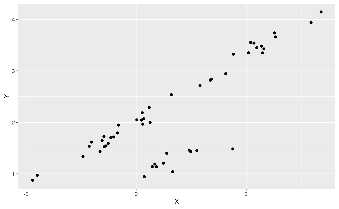

summary(lm(Y~X,df))
#> 
#> Call:
#> lm(formula = Y ~ X, data = df)
#> 
#> Residuals:
#>      Min       1Q   Median       3Q      Max 
#> -1.37351  0.08688  0.21850  0.31787  0.49193 
#> 
#> Coefficients:
#>             Estimate Std. Error t value Pr(>|t|)    
#> (Intercept)  1.76503    0.08313   21.23  < 2e-16 ***
#> X            0.24886    0.02369   10.50 4.96e-14 ***
#> ---
#> Signif. codes:  0 '***' 0.001 '**' 0.01 '*' 0.05 '.' 0.1 ' ' 1
#> 
#> Residual standard error: 0.5224 on 48 degrees of freedom
#> Multiple R-squared:  0.6968, Adjusted R-squared:  0.6905 
#> F-statistic: 110.3 on 1 and 48 DF,  p-value: 4.955e-14

################################################################################################################
#Simulate errors 
Z_X_error<-1 #Number of X traits with error
X_error<-rep(0.01,N)
Y_error<-rep(0.01,N)
Y_with_error<-Y+rnorm(N,0,0.01)
X_with_error<-X+rnorm(N,0,0.01)

############################################################################################################
#Make trdata file
trdata$dat<-cbind(trdata$dat,data.frame(cbind(Y_with_error,Y_error,X_with_error,X_error)))

Next we will set the priors for the estimated parameters - for this model this includes the half-life, Vy, optima, and beta. For the latter two parameters we will use the results of the linear model to inform our priors.

############################################################################################################
#Set Priors
hl.prior<-c(log(0.25),0.75)
vy.prior<-5
optima.prior<-c(1.5,0.5) #Informed by linear model
beta.prior<-c(0,0.25)

Exploring Priors

At this point one would want to explore if the priors are appropriate - do the prior distributions look consistent with what we know about our system? See Grabowski (in press) for more on setting priors.

Half-life Prior plot

hl.sims<-data.frame(rlnorm(n=1000,meanlog=hl.prior[1],sdlog=hl.prior[2]))
names(hl.sims)<-"prior.hl.sims"

hl.prior.plot<-ggplot2::ggplot()+
  ggplot2::geom_density(ggplot2::aes(prior.hl.sims,fill="prior.hl.sims"),alpha=0.2,data=hl.sims)+
  ggplot2::theme_bw()+
  ggplot2::theme(
    panel.grid.major = ggplot2::element_blank(),
    panel.grid.minor = ggplot2::element_blank())+
  
  #labs(title="Prior vs. Posterior Distribution ",x="Half-life", y = "Density")+
  ggplot2::labs(title="",x="Half-life", y = "Density")+
  
  #scale_fill_manual(labels=c("Posterior","Prior"))+
  ggplot2::geom_vline(xintercept=c(hl),linetype=2)+
  ggsci::scale_fill_npg(name="",labels=c("Prior"))

hl.prior.plot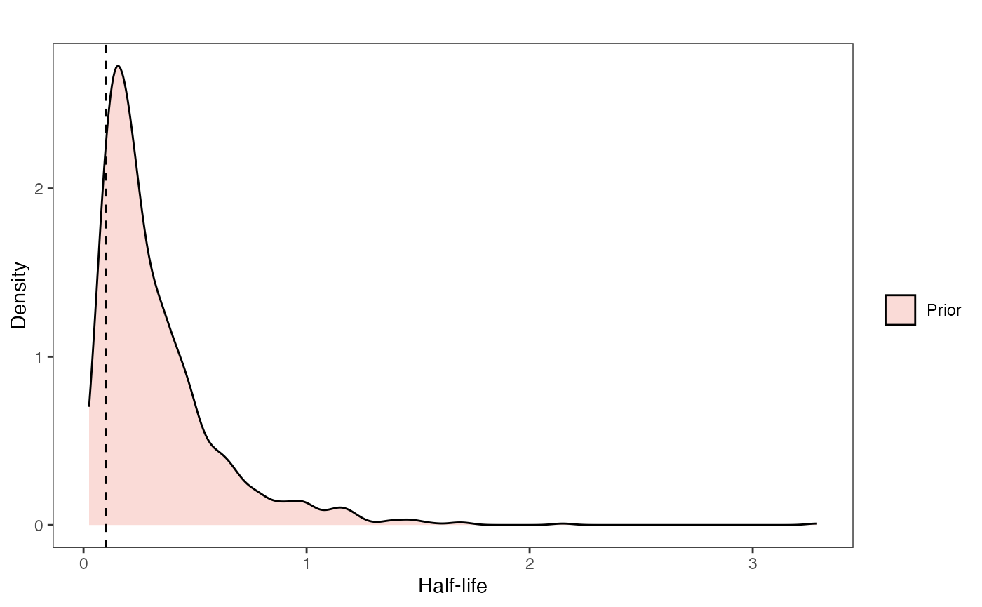

Vy Prior Plot

vy.sims<-rexp(n=1000,rate=vy.prior)
vy.sims<-data.frame(vy.sims)
names(vy.sims)<-"prior.vy.sims"

vy.prior.plot<-ggplot2::ggplot()+
  ggplot2::geom_density(ggplot2::aes(prior.vy.sims,fill="prior.vy.sims"),alpha=0.2,data=vy.sims)+
  ggplot2::theme_bw()+
  ggplot2::theme(
    panel.grid.major = ggplot2::element_blank(),
    panel.grid.minor = ggplot2::element_blank())+
  
  #labs(title="Prior vs. Posterior Distribution ",x="vy", y = "Density")+
  ggplot2::labs(title="",x="vy", y = "Density")+
  ggplot2::geom_vline(xintercept=c(vy),linetype=2)+
  
  #scale_fill_manual(labels=c("Posterior","Prior"))+
  ggsci::scale_fill_npg(name="",labels=c("Prior"))


vy.prior.plot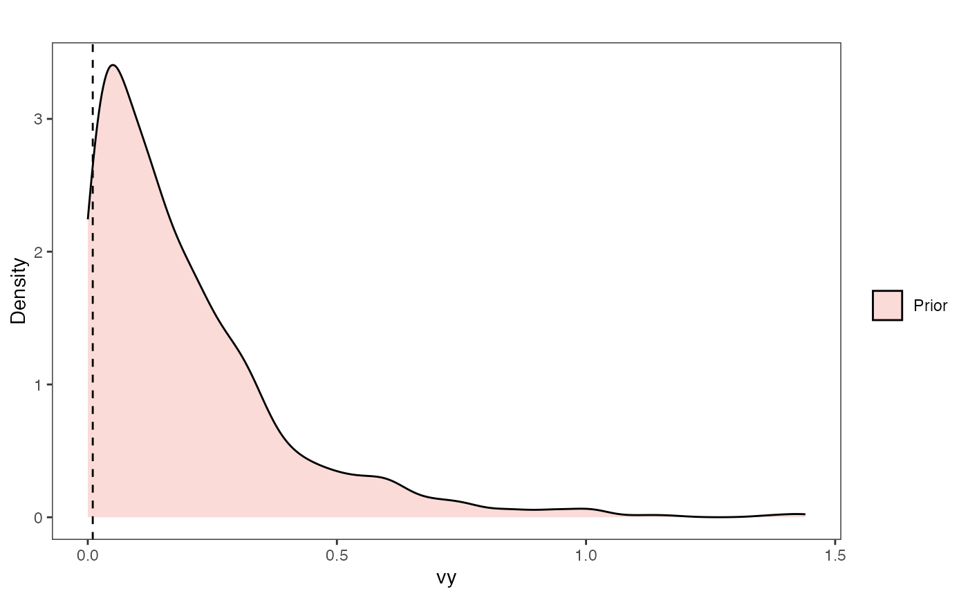

Prior on how shared branch lengths correspond to covariance

a.sims<-log(2)/hl.sims;
sigma2_y.sims<-vy.sims*(2*(log(2)/hl.sims));

plot( NULL , xlim=c(0,1) , ylim=c(0,1) , xlab="Time since MRCA" , ylab="Covariance" ,cex.axis=0.75, mgp=c(1.25,0.25,0),tcl=-0.25)
for (i in 1:30){
  curve(sigma2_y.sims[i,] /(2 * a.sims[i,]) * ((1 - exp(-2 * a.sims[i,] * (1-(x/2)))) * exp(-a.sims[i,] * x)) , add=TRUE , lwd=4 , col=rethinking::col.alpha(1,0.15))
}

par(mar=c(3,3,0.25,0.25))
covariance.prior.plot <- recordPlot()
dev.off()
#> null device 
#>           1
covariance.prior.plot

Slope and intercept Prior Plot

optima.sims<-rnorm(100,optima.prior[1],optima.prior[2])
beta.sims<-rnorm(n=100,beta.prior[1],beta.prior[2])

prior.slope.plot<-ggplot2::ggplot()+  
 ggplot2:: geom_point(data=df,ggplot2::aes(y=Y,x=X))+
  ggplot2::geom_abline(intercept=optima.sims,slope=beta.sims,alpha=0.15)+
  ggplot2::theme_bw()+
  ggplot2::theme(
    panel.grid.major = ggplot2::element_blank(),
    panel.grid.minor = ggplot2::element_blank())+
  
  ggplot2::ylab("Trait 1") + ggplot2::xlab("Trait 2")+
  ggsci::scale_color_npg()

prior.slope.plot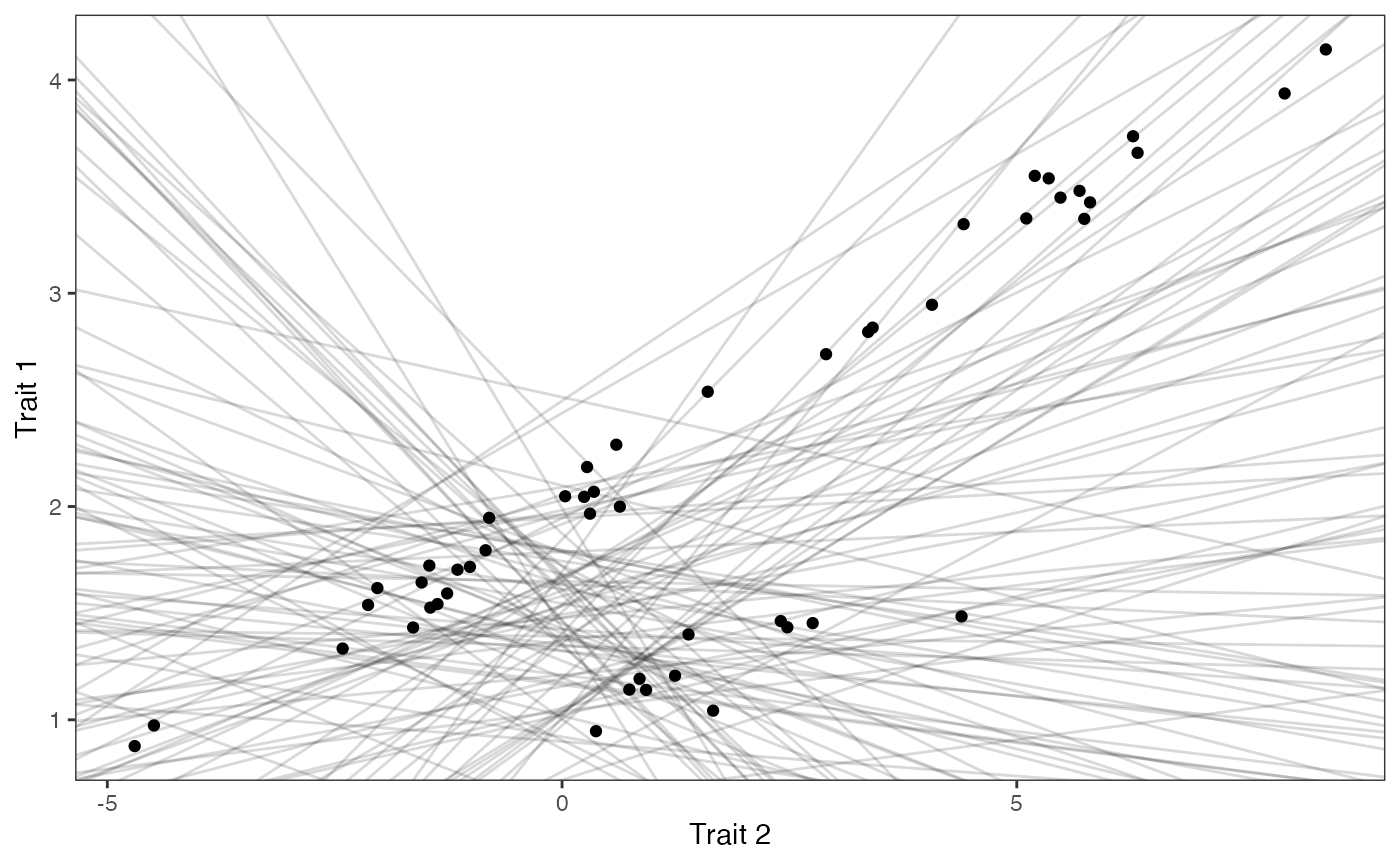

We will use the helper function blouch.reg.direct.prep() to setup the dat file for Stan. Here “Z_direct” is the number of predictors, and “regimes” is the name of the regime column in trdata$dat.

############################################################################################################
#Blouch prep code - Regimes + Direct Efffect model
#source("/Users/markgrabowski/Documents/Academic/Research/Current Projects/Blouch project/blouch/R Setup Code/blouch.prep.R")
dat<-blouch.reg.direct.prep(trdata,"Y_with_error","Y_error","X_with_error","X_error",Z_direct=1,"regimes",hl.prior,vy.prior,optima.prior,beta.prior)

Multi-optima Direct Effect Model with Varying Effects

fit.reg.direct.ve<- rstan::sampling(object = blouch:::stanmodels$blouchOU_reg_direct_ve,data = dat,chains = 2,cores=2,iter =2000)
#> Found more than one class "stanfit" in cache; using the first, from namespace 'rstan'
#> Also defined by 'rethinking'
#> Found more than one class "stanfit" in cache; using the first, from namespace 'rstan'
#> Also defined by 'rethinking'

print(fit.reg.direct.ve,pars = c("hl","vy","optima","beta"))
#> Inference for Stan model: blouchOU_reg_direct_ve.
#> 2 chains, each with iter=2000; warmup=1000; thin=1; 
#> post-warmup draws per chain=1000, total post-warmup draws=2000.
#> 
#>           mean se_mean   sd 2.5%  25%  50%  75% 97.5% n_eff Rhat
#> hl        0.16       0 0.09 0.06 0.10 0.14 0.20  0.37  1106    1
#> vy        0.02       0 0.01 0.01 0.01 0.02 0.02  0.03   973    1
#> optima[1] 2.01       0 0.04 1.92 1.98 2.01 2.03  2.09  2242    1
#> optima[2] 0.98       0 0.11 0.69 0.92 0.99 1.06  1.17  1326    1
#> beta[1,1] 0.26       0 0.01 0.24 0.25 0.26 0.26  0.27  3028    1
#> beta[2,1] 0.13       0 0.03 0.07 0.11 0.13 0.15  0.19  3065    1
#> 
#> Samples were drawn using NUTS(diag_e) at Tue Oct  8 14:10:55 2024.
#> For each parameter, n_eff is a crude measure of effective sample size,
#> and Rhat is the potential scale reduction factor on split chains (at 
#> convergence, Rhat=1).
post<-rstan::extract(fit.reg.direct.ve)

Now lets look at the prior vs. posterior plots for the parameters Half-life plot

hl.post<-data.frame(post$hl)
names(hl.post)<-"post.hl.sims"

hl.plot<-ggplot2::ggplot()+
  ggplot2::geom_density(ggplot2::aes(prior.hl.sims,fill="prior.hl.sims"),alpha=0.2,data=hl.sims)+
  ggplot2::geom_density(ggplot2::aes(post.hl.sims,fill="post.hl.sims"),alpha=0.2,data=hl.post)+
  ggplot2::theme_bw()+
  ggplot2::theme(
    panel.grid.major = ggplot2::element_blank(),
    panel.grid.minor = ggplot2::element_blank())+
  
  #labs(title="Prior vs. Posterior Distribution ",x="Half-life", y = "Density")+
  ggplot2::labs(title="",x="Half-life", y = "Density")+
  
  #scale_fill_manual(labels=c("Posterior","Prior"))+
  ggplot2::geom_vline(xintercept=c(hl),linetype=2)+
  ggsci::scale_fill_npg(name="",labels=c("Posterior","Prior"))

hl.plot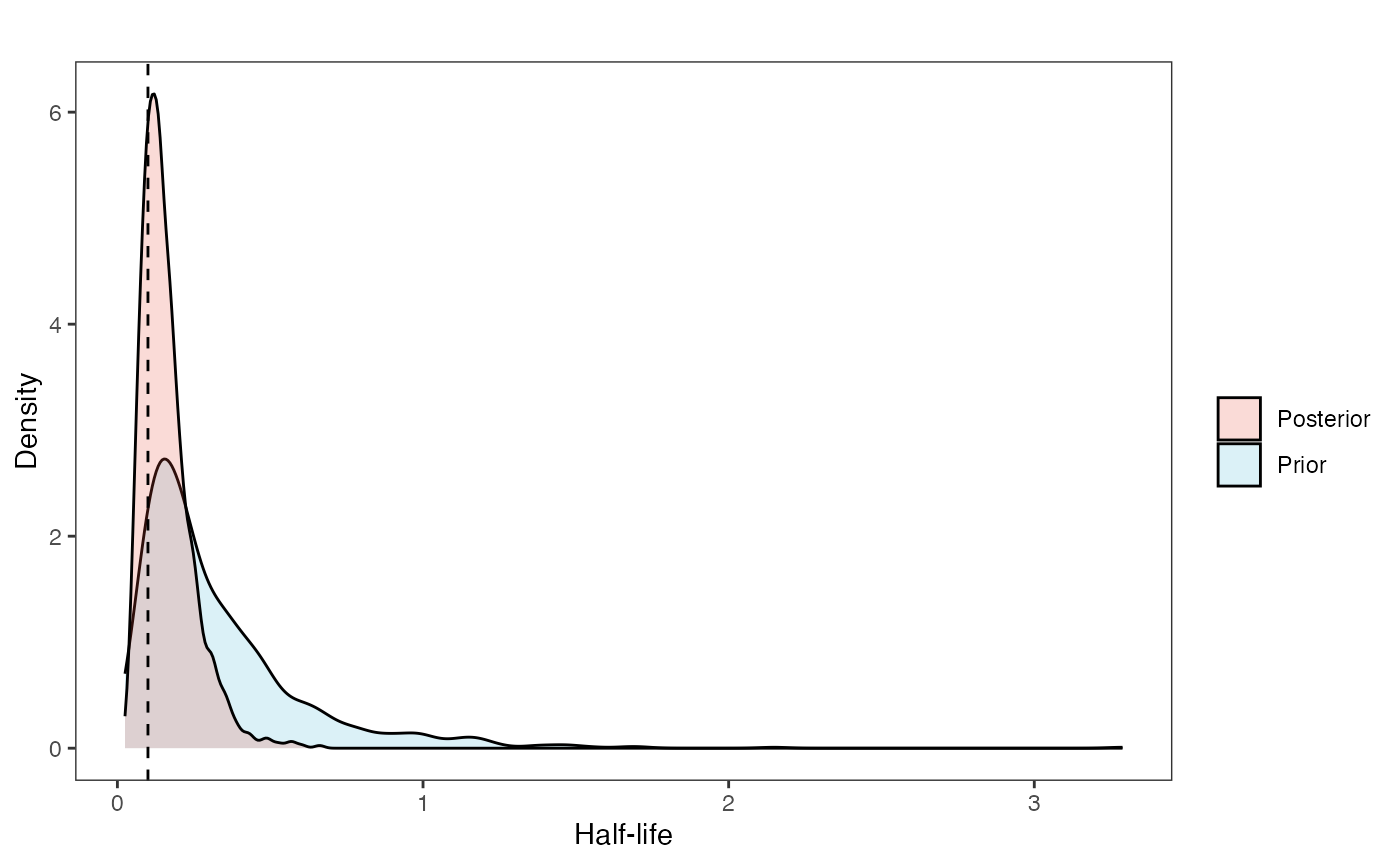

Vy Prior vs. posterior plot

vy.post<-data.frame(post$vy)
names(vy.post)<-"post.vy.sims"


vy.plot<-ggplot2::ggplot()+
  ggplot2::geom_density(ggplot2::aes(prior.vy.sims,fill="prior.vy.sims"),alpha=0.2,data=vy.sims)+
  ggplot2::geom_density(ggplot2::aes(post.vy.sims,fill="post.vy.sims"),alpha=0.2,data=vy.post)+
  ggplot2::theme_bw()+
  ggplot2::theme(
    panel.grid.major = ggplot2::element_blank(),
    panel.grid.minor = ggplot2::element_blank())+
  
  #labs(title="Prior vs. Posterior Distribution ",x="vy", y = "Density")+
  ggplot2::labs(title="",x="vy", y = "Density")+
  ggplot2::geom_vline(xintercept=c(vy),linetype=2)+
  
  #scale_fill_manual(labels=c("Posterior","Prior"))+
  ggsci::scale_fill_npg(name="",labels=c("Posterior","Prior"))

vy.plot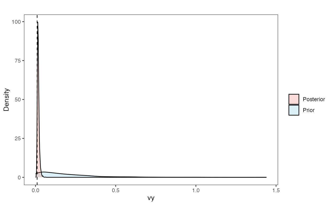

Prior versus posterior on how shared branch lengths correspond to covariance

plot( NULL , xlim=c(0,1) , ylim=c(0,1) , xlab="Time since MRCA" , ylab="Covariance" ,cex.axis=0.75, mgp=c(1.25,0.25,0),tcl=-0.25)
for (i in 1:30){
  curve(sigma2_y.sims[i,] /(2 * a.sims[i,]) * ((1 - exp(-2 * a.sims[i,] * (1-(x/2)))) * exp(-a.sims[i,] * x)) , add=TRUE , lwd=4 , col=rethinking::col.alpha(1,0.15))
}

for (i in 1:30){
  curve(post$sigma2_y[i] /(2 * post$a[i]) * ((1 - exp(-2 * post$a[i] * (1-(x/2)))) * exp(-post$a[i] * x)) , add=TRUE , lwd=4 , col=rethinking::col.alpha(2,0.5))
}

par(mar=c(3,3,0.25,0.25))
covariance.plot <- recordPlot()
dev.off()
#> null device 
#>           1
covariance.plot

Prior vs. Posterior Plot for Regression

optima.sims<-rnorm(100,optima.prior[1],optima.prior[2])
beta.sims<-rnorm(n=100,beta.prior[1],beta.prior[2])

optima.post<-post$optima
beta.post<-data.frame(post$beta)
names(beta.post)<-c("post.beta.1","post.beta.2")

mu.link.11<-function(x.seq){optima.post[,1]+x.seq*beta.post[,1]}
mu.link.12<-function(x.seq){optima.post[,2]+x.seq*beta.post[,2]}

x.seq <- seq(from=min(X), to=max(X) , length.out=100)
mu.11 <- sapply(x.seq , mu.link.11 )
mu.12 <- sapply(x.seq , mu.link.12 )


mu.mean.11<-colMeans(mu.11)
mu.mean.12<-colMeans(mu.12)

mu.mean.11<-data.frame(as.numeric(mu.mean.11))
mu.mean.12<-data.frame(as.numeric(mu.mean.12))
names(mu.mean.11)<-"mu.mean.11"
names(mu.mean.12)<-"mu.mean.12"

mu.CI.11 <- apply( mu.11 , MARGIN=2, FUN=rethinking::PI , prob=0.89 )
mu.CI.12 <- apply( mu.12 , MARGIN=2, FUN=rethinking::PI , prob=0.89 )

mu.CI.11<-data.frame(t(data.frame(mu.CI.11)),x.seq)
mu.CI.12<-data.frame(t(data.frame(mu.CI.12)),x.seq)

names(mu.CI.11)<-c("min.5.5","max.94.5","x.seq")
names(mu.CI.12)<-c("min.5.5","max.94.5","x.seq")

df<-data.frame(Y=dat$Y_obs,X=dat$X_obs,Regimes=regimes_tip)
df11<-data.frame(x.seq,mu.mean.11)
df12<-data.frame(x.seq,mu.mean.12)


slope.plot.1<-ggplot2::ggplot()+  
  ggplot2::geom_point(data=df,ggplot2::aes(y=Y,x=X,color=Regimes))+
  ggplot2::geom_abline(intercept=optima.sims,slope=beta.sims,alpha=0.1)+
  
  ggplot2::geom_abline(intercept=optima[1],slope=beta[1],alpha=0.5,linetype=2)+
  ggplot2::geom_abline(intercept=optima[2],slope=beta[2],alpha=0.5,linetype=2)+
  
  ggplot2::geom_line(data=df11,ggplot2::aes(x=x.seq,y=mu.mean.11),linetype=1)+
  ggplot2::geom_ribbon(data=mu.CI.11,ggplot2::aes(x=x.seq,ymin=min.5.5,ymax=max.94.5),linetype=2,alpha=0.25)+
  ggplot2::geom_line(data=df12,ggplot2::aes(x=x.seq,y=mu.mean.12),linetype=1)+
  ggplot2::geom_ribbon(data=mu.CI.12,ggplot2::aes(x=x.seq,ymin=min.5.5,ymax=max.94.5),linetype=2,alpha=0.25)+
  
  ggplot2::theme_bw()+
  ggplot2::theme(
  panel.grid.major = ggplot2::element_blank(),
  panel.grid.minor = ggplot2::element_blank())+
  
  ggplot2::ylab("Y") + ggplot2::xlab("Direct effect trait")+
  ggsci::scale_color_npg()

slope.plot.1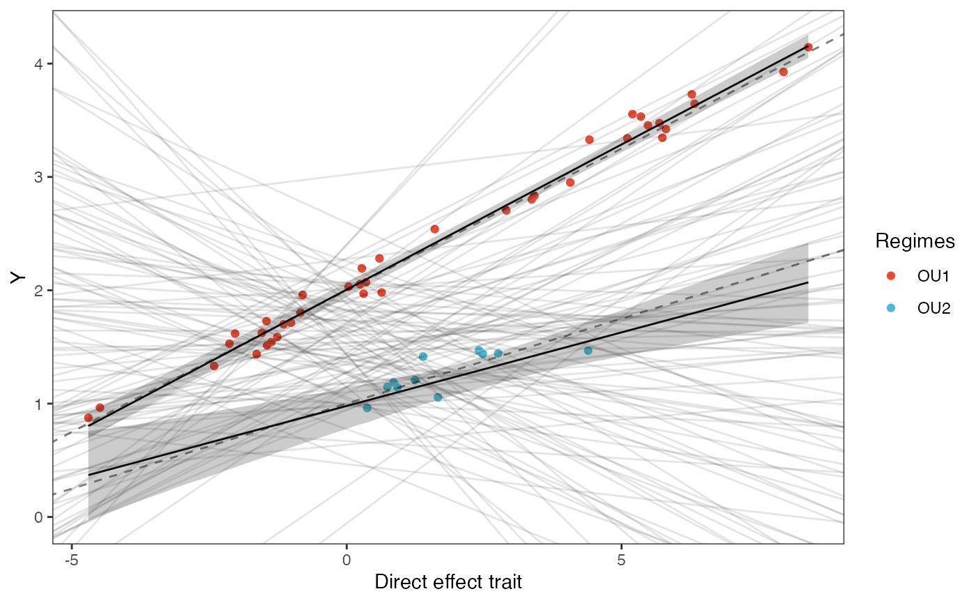

`Multilevel Multi-optima Direct Effect Model with Varying Effects

Next we will set the priors for the estimated parameters - for this model this includes the half-life, Vy, optima, and beta. For the latter two parameters we will use the results of the linear model to inform our priors.

############################################################################################################
#Set Priors
hl.prior<-c(log(0.25),0.75)
vy.prior<-5
optima.prior<-c(1.5,0.5) #Informed by linear model
beta.prior<-c(0,0.25)
sigma.prior<-c(0,1)

We will use the helper function blouch.reg.direct.prep() to setup the dat file for Stan. Here “Z_direct” is the number of predictors, and “regimes” is the name of the regime column in trdata$dat.

############################################################################################################
dat<-blouch.reg.direct.mlm.prep(trdata,"Y_with_error","Y_error","X_with_error","X_error",Z_direct=1,"regimes",hl.prior,vy.prior,optima.prior,beta.prior,sigma.prior)

fit.reg.direct.mlm.ve<- rstan::sampling(object = blouch:::stanmodels$blouchOU_reg_direct_mlm_ve,data = dat,chains = 2,cores=2,iter=2000)
#> Found more than one class "stanfit" in cache; using the first, from namespace 'rstan'
#> Also defined by 'rethinking'
#> Found more than one class "stanfit" in cache; using the first, from namespace 'rstan'
#> Also defined by 'rethinking'
#> Warning: There were 25 divergent transitions after warmup. See
#> https://mc-stan.org/misc/warnings.html#divergent-transitions-after-warmup
#> to find out why this is a problem and how to eliminate them.
#> Warning: Examine the pairs() plot to diagnose sampling problems

print(fit.reg.direct.mlm.ve,pars = c("hl","vy","optima_bar","beta_bar","Rho","sigma","optima","beta"))
#> Inference for Stan model: blouchOU_reg_direct_mlm_ve.
#> 2 chains, each with iter=2000; warmup=1000; thin=1; 
#> post-warmup draws per chain=1000, total post-warmup draws=2000.
#> 
#>             mean se_mean   sd  2.5%   25%  50%  75% 97.5% n_eff Rhat
#> hl          0.18    0.01 0.13  0.05  0.10 0.15 0.22  0.51   196 1.01
#> vy          0.02    0.00 0.01  0.01  0.01 0.02 0.02  0.04   195 1.01
#> optima_bar  1.49    0.01 0.38  0.74  1.26 1.48 1.73  2.25  1998 1.00
#> beta_bar[1] 0.12    0.01 0.17 -0.29  0.04 0.16 0.22  0.39  1087 1.00
#> Rho[1,1]    1.00     NaN 0.00  1.00  1.00 1.00 1.00  1.00   NaN  NaN
#> Rho[1,2]    0.07    0.01 0.33 -0.59 -0.16 0.08 0.32  0.67  2602 1.00
#> Rho[2,1]    0.07    0.01 0.33 -0.59 -0.16 0.08 0.32  0.67  2602 1.00
#> Rho[2,2]    1.00    0.00 0.00  1.00  1.00 1.00 1.00  1.00  1939 1.00
#> sigma[1]    0.86    0.01 0.40  0.33  0.56 0.76 1.06  1.83  1589 1.00
#> sigma[2]    0.34    0.01 0.34  0.04  0.11 0.23 0.43  1.26  1131 1.00
#> optima[1]   2.01    0.00 0.04  1.92  1.98 2.01 2.03  2.09  1561 1.00
#> optima[2]   0.94    0.01 0.19  0.49  0.89 0.97 1.04  1.14   186 1.01
#> beta[1,1]   0.26    0.00 0.01  0.24  0.25 0.26 0.26  0.27  2053 1.00
#> beta[2,1]   0.14    0.00 0.04  0.07  0.11 0.14 0.16  0.21  1554 1.00
#> 
#> Samples were drawn using NUTS(diag_e) at Tue Oct  8 14:11:23 2024.
#> For each parameter, n_eff is a crude measure of effective sample size,
#> and Rhat is the potential scale reduction factor on split chains (at 
#> convergence, Rhat=1).
post<-rstan::extract(fit.reg.direct.mlm.ve)

Multilevel Multi-optima Direct Effect Model with Varying Effects - Non centered

fit.reg.direct.mlm.ve.nc<- rstan::sampling(object = blouch:::stanmodels$blouchOU_reg_direct_mlm_ve_nc,data = dat,chains = 2,cores=2,iter=2000)
#> Found more than one class "stanfit" in cache; using the first, from namespace 'rstan'
#> Also defined by 'rethinking'
#> Found more than one class "stanfit" in cache; using the first, from namespace 'rstan'
#> Also defined by 'rethinking'
#> Warning: There were 506 divergent transitions after warmup. See
#> https://mc-stan.org/misc/warnings.html#divergent-transitions-after-warmup
#> to find out why this is a problem and how to eliminate them.
#> Warning: Examine the pairs() plot to diagnose sampling problems
#> Warning: The largest R-hat is NA, indicating chains have not mixed.
#> Running the chains for more iterations may help. See
#> https://mc-stan.org/misc/warnings.html#r-hat
#> Warning: Bulk Effective Samples Size (ESS) is too low, indicating posterior means and medians may be unreliable.
#> Running the chains for more iterations may help. See
#> https://mc-stan.org/misc/warnings.html#bulk-ess
#> Warning: Tail Effective Samples Size (ESS) is too low, indicating posterior variances and tail quantiles may be unreliable.
#> Running the chains for more iterations may help. See
#> https://mc-stan.org/misc/warnings.html#tail-ess

print(fit.reg.direct.mlm.ve.nc,pars = c("hl","vy","optima_bar","beta_bar","Rho","sigma","optima","beta"))
#> Inference for Stan model: blouchOU_reg_direct_mlm_ve_nc.
#> 2 chains, each with iter=2000; warmup=1000; thin=1; 
#> post-warmup draws per chain=1000, total post-warmup draws=2000.
#> 
#>            mean se_mean   sd  2.5%   25%  50%  75% 97.5% n_eff Rhat
#> hl         0.17    0.01 0.10  0.06  0.11 0.14 0.19  0.44   140 1.02
#> vy         0.02    0.00 0.01  0.01  0.01 0.02 0.02  0.03    96 1.02
#> optima_bar 1.48    0.01 0.33  0.79  1.33 1.47 1.65  2.15  1019 1.00
#> beta_bar   0.16    0.01 0.12 -0.15  0.11 0.19 0.24  0.38    80 1.02
#> Rho[1,1]   1.00     NaN 0.00  1.00  1.00 1.00 1.00  1.00   NaN  NaN
#> Rho[1,2]   0.09    0.01 0.29 -0.50 -0.10 0.14 0.26  0.63  1599 1.00
#> Rho[2,1]   0.09    0.01 0.29 -0.50 -0.10 0.14 0.26  0.63  1599 1.00
#> Rho[2,2]   1.00    0.00 0.00  1.00  1.00 1.00 1.00  1.00  1062 1.00
#> sigma[1]   0.83    0.04 0.39  0.32  0.57 0.70 1.00  1.88    81 1.03
#> sigma[2]   0.35    0.09 0.29  0.04  0.11 0.24 0.57  0.91     9 1.16
#> optima[1]  2.01    0.00 0.04  1.93  1.98 2.01 2.03  2.09   645 1.00
#> optima[2]  0.97    0.02 0.14  0.58  0.91 0.99 1.05  1.17    82 1.02
#> beta[1,1]  0.26    0.00 0.01  0.24  0.25 0.26 0.26  0.27  1176 1.00
#> beta[2,1]  0.13    0.00 0.04  0.06  0.11 0.13 0.16  0.21   133 1.01
#> 
#> Samples were drawn using NUTS(diag_e) at Tue Oct  8 14:13:18 2024.
#> For each parameter, n_eff is a crude measure of effective sample size,
#> and Rhat is the potential scale reduction factor on split chains (at 
#> convergence, Rhat=1).
post<-rstan::extract(fit.reg.direct.mlm.ve.nc)

rm(list=ls())

Multlevel Multi-optima Direct Effect Model with Varying Effects - Multiple Predictors

Two regimes with two direct effect predictors and multiple slopes per optima but single alpha parameter

############################################################################################################
#Regimes model
############################################################################################################
########################################################################################################
#Create phylogeny
########################################################################################################
N<-50 #Number of species
set.seed(10) #Set seed to get same random species each time

phy <- ape::keep.tip(tree.10K,sample(tree.10K$tip.label)[1:N]) 
phy<-ape::multi2di(phy)

l.tree<-max(ape::branching.times(phy)) ## rescale tree to height 1
phy$edge.length<-phy$edge.length/l.tree 

tip.label<-phy$tip.label


#Set regimes - manually - 2 regimes
#Locate nodes
plot(phy,no.margin=TRUE,edge.width=2,cex=0.7)
ape::nodelabels(frame="none",adj=c(1.1,-0.4))
ape::tiplabels()

#Paint Regimes on Tree
#source("/Users/markgrabowski/Documents/Academic/Research/Current Projects/Blouch project/blouch/Simulation Code/Functions/set.converge.regimes.R") #Macbook Pro

shifts<-c(84) #Location of nodes with regime shifts
trdata<-data.frame(phy$tip.label)
trdata<-treeplyr::make.treedata(phy,trdata)
trdata<-set.converge.regimes(trdata,shifts)
#> [1] 1
#>  [1] OU1 OU1 OU1 OU1 OU1 OU1 OU1 OU1 OU1 OU1 OU1 OU1 OU1 OU1 OU1 OU1 OU1 OU1 OU1
#> [20] OU1 OU1 OU1 OU1 OU1 OU1 OU1 OU1 OU1 OU1 OU1 OU1 OU1 OU1 OU1 OU1 OU1 OU1 OU1
#> [39] OU1 OU1 OU1 OU1 OU1 OU1 OU1 OU1 OU1 OU1 OU1 OU1 OU1 OU1 OU1 OU1 OU1 OU1 OU1
#> [58] OU1 OU1 OU1 OU1 OU1 OU1 OU1 OU2 OU2 OU2 OU2 OU2 OU2 OU2 OU2 OU2 OU2 OU2 OU2
#> [77] OU2 OU2 OU2 OU2 OU2 OU2 OU2 OU2 OU2 OU1 OU1 OU1 OU1 OU1 OU1 OU1 OU1 OU1 OU1
#> [96] OU1 OU1 OU1
#> Levels: OU1 OU2
#> [1] "#E64B35FF" "#4DBBD5FF"

#Check if manual setting code worked
shifts.total<-c(trdata$dat$regimes,trdata$phy$node.label)
edge.regimes <- factor(shifts.total[trdata$phy$edge[,2]])
print(edge.regimes)
#>  [1] OU1 OU1 OU1 OU1 OU1 OU1 OU1 OU1 OU1 OU1 OU1 OU1 OU1 OU1 OU1 OU1 OU1 OU1 OU1
#> [20] OU1 OU1 OU1 OU1 OU1 OU1 OU1 OU1 OU1 OU1 OU1 OU1 OU1 OU1 OU1 OU1 OU1 OU1 OU1
#> [39] OU1 OU1 OU1 OU1 OU1 OU1 OU1 OU1 OU1 OU1 OU1 OU1 OU1 OU1 OU1 OU1 OU1 OU1 OU1
#> [58] OU1 OU1 OU1 OU1 OU1 OU1 OU1 OU2 OU2 OU2 OU2 OU2 OU2 OU2 OU2 OU2 OU2 OU2 OU2
#> [77] OU2 OU2 OU2 OU2 OU2 OU2 OU2 OU2 OU2 OU1 OU1 OU1 OU1 OU1 OU1 OU1 OU1 OU1 OU1
#> [96] OU1 OU1 OU1
#> Levels: OU1 OU2

reg_tips<-trdata$dat$regimes
reg_tips<-as.numeric(as.factor(reg_tips))

reg.colors <- ggsci::pal_aaas("default", alpha = 0.7)(2)
print(reg.colors)
#> [1] "#3B4992B2" "#EE0000B2"
plot(trdata$phy,edge.color = reg.colors[edge.regimes], edge.width = 1, cex = 0.2)

Format tree

############################################################################################################
#Simulate data
n<-length(trdata$phy$tip.label)
regimes_internal <-trdata$phy$node.label
regimes_tip <- trdata$dat$regimes
regimes <- concat.factor(regimes_tip, regimes_internal)
anc_maps<-"regimes"
lineages <- lapply(1:n, function(e) lineage.constructor(trdata$phy, e, anc_maps, regimes)) #Trace lineage from tips (n) to root and determine regimes of each node or branch

Simulate two direct effect traits

#########################
hl<-0.1 #0.1, 0.25, 0.75 - testing options
a<-log(2)/hl
vy<-0.01 #0.25,0.5 - testing options
sigma2_y<-vy*(2*(log(2)/hl));

vX0<-0
vY0 <- 0
Sxx<-10 #Look at effects

Z_direct<-2
vcv<-matrix(c(1,0,0,1),2,2) #No correlation between traits
Xs<-phytools::sim.corrs(phy,vcv) #Simulated correlated BM Xs

phytools::phenogram(phy,Xs[,1],spread.labels=TRUE,spread.cost=c(1,0)) #Plot X data
#> Optimizing the positions of the tip labels...

phytools::phenogram(phy,Xs[,2],spread.labels=TRUE,spread.cost=c(1,0)) #Plot X data
#> Optimizing the positions of the tip labels...

dmX<-weight.matrix(trdata$phy, a, lineages) #Slouch approach
optima<-c(2,1)
beta<-data.frame(matrix(c(0.25,0.15,0.35,0.1),ncol=2,nrow=2)) #Two traits on columns, two regimes on vertical

mu<-matrix(NA,N,1)
for(i in 1:N){
  mu[i]<-dmX[i,]%*%optima+Xs[i,]%*%t(beta[reg_tips[i],]);
}

V<-calc_direct_V(phy,sigma2_y,a)
Y<-MASS::mvrnorm(n=1,mu,V)


###############################################################################################################

summary(lm(Y~Xs))
#> 
#> Call:
#> lm(formula = Y ~ Xs)
#> 
#> Residuals:
#>      Min       1Q   Median       3Q      Max 
#> -0.71025 -0.12589  0.09583  0.17052  0.62782 
#> 
#> Coefficients:
#>             Estimate Std. Error t value Pr(>|t|)    
#> (Intercept)  2.08067    0.06724  30.944  < 2e-16 ***
#> Xs1          0.14691    0.04486   3.275  0.00199 ** 
#> Xs2          0.57128    0.05648  10.114 2.22e-13 ***
#> ---
#> Signif. codes:  0 '***' 0.001 '**' 0.01 '*' 0.05 '.' 0.1 ' ' 1
#> 
#> Residual standard error: 0.2912 on 47 degrees of freedom
#> Multiple R-squared:  0.771,  Adjusted R-squared:  0.7612 
#> F-statistic:  79.1 on 2 and 47 DF,  p-value: 9.077e-16

################################################################################################################


################################################################################################################
#Simulate errors 
Z_X_error<-2 #Number of X traits with error
X_error<-matrix(0.01,nrow=N,ncol=Z_X_error)
X_error<-data.frame(X_error)
names(X_error)<-c("X1_error","X2_error")
Y_error<-rep(0.01,N)
Y_with_error<-Y+rnorm(N,0,0.01)
X_with_error<-Xs+rnorm(N,0,0.01)
X_with_error<-data.frame(X_with_error)
names(X_with_error)<-c("X1","X2")
############################################################################################################
#Make trdata file
trdata$dat<-cbind(trdata$dat,data.frame(cbind(Y_with_error,Y_error,X_with_error,X_error)))

Next we will set the priors for the estimated parameters - for this model this includes the half-life, Vy, optima, and beta. For the latter two parameters we will use the results of the linear model to inform our priors.

############################################################################################################
#Set Priors
hl.prior<-c(log(0.25),0.75)
vy.prior<-5
optima.prior<-c(1.5,0.5) #Informed by linear model
beta.prior<-c(0,0.25)

We will use the helper function blouch.reg.direct.prep() to setup the dat file for Stan. Here “Z_direct” is the number of predictors, and “regimes” is the name of the regime column in trdata$dat.

############################################################################################################
#Test Blouch prep code - Regimes + Direct Efffect model
dat<-blouch.reg.direct.prep(trdata,"Y_with_error","Y_error",c("X1","X2"),c("X1_error","X2_error"),Z_direct=2,"regimes",hl.prior,vy.prior,optima.prior,beta.prior)

Multi-optima Direct Efect Model with Varying Effects

fit.reg.direct.ve<- rstan::sampling(object = blouch:::stanmodels$blouchOU_reg_direct_ve,data = dat,chains = 2,cores=2,iter =2000)
#> Found more than one class "stanfit" in cache; using the first, from namespace 'rstan'
#> Also defined by 'rethinking'
#> Found more than one class "stanfit" in cache; using the first, from namespace 'rstan'
#> Also defined by 'rethinking'

print(fit.reg.direct.ve,pars = c("hl","vy","optima","beta"))
#> Inference for Stan model: blouchOU_reg_direct_ve.
#> 2 chains, each with iter=2000; warmup=1000; thin=1; 
#> post-warmup draws per chain=1000, total post-warmup draws=2000.
#> 
#>           mean se_mean   sd 2.5%  25%  50%  75% 97.5% n_eff Rhat
#> hl        0.17       0 0.09 0.06 0.11 0.15 0.21  0.41   606    1
#> vy        0.01       0 0.00 0.01 0.01 0.01 0.01  0.02   577    1
#> optima[1] 2.05       0 0.04 1.97 2.02 2.05 2.07  2.12  1341    1
#> optima[2] 1.00       0 0.14 0.72 0.92 1.01 1.09  1.25   826    1
#> beta[1,1] 0.22       0 0.02 0.17 0.20 0.22 0.23  0.26  1587    1
#> beta[1,2] 0.33       0 0.03 0.27 0.31 0.33 0.35  0.39  1482    1
#> beta[2,1] 0.27       0 0.08 0.10 0.22 0.27 0.33  0.44  1870    1
#> beta[2,2] 0.19       0 0.07 0.05 0.14 0.19 0.23  0.33  1142    1
#> 
#> Samples were drawn using NUTS(diag_e) at Tue Oct  8 14:13:44 2024.
#> For each parameter, n_eff is a crude measure of effective sample size,
#> and Rhat is the potential scale reduction factor on split chains (at 
#> convergence, Rhat=1).
#plot(rethinking::precis(fit.reg.direct.ve,depth=3,pars = c("hl","vy","optima","beta")))
post<-rstan::extract(fit.reg.direct.ve)

From there the posteriors should be explored, compared to the priors, etc. One can also use the varying effects and multilevel models on multiple predictors in the same fashion as above.

rm(list=ls())

Multlevel Multi-optima Adaptive Model with Varying Effects - Single Predictor

########################################################################################################
#Two regimes with adaptive trait and multiple slopes per optima but single alpha parameter
set.seed(10)
N<-50 #Number of species
#set.seed(1) #Set seed to get same random species each time

phy <- ape::keep.tip(tree.10K,sample(tree.10K$tip.label)[1:N]) 
phy<-ape::multi2di(phy)

l.tree<-max(ape::branching.times(phy)) ## rescale tree to height 1
phy$edge.length<-phy$edge.length/l.tree 

#Set regimes - manually - 2 regimes
#Locate nodes
plot(phy,no.margin=TRUE,edge.width=2,cex=0.7)
ape::nodelabels(frame="none",adj=c(1.1,-0.4))
ape::tiplabels()

#Paint Regimes on Tree
shifts<-c(84) #Location of nodes with regime shifts
trdata<-data.frame(phy$tip.label)
trdata<-treeplyr::make.treedata(phy,trdata)
trdata<-set.converge.regimes(trdata,shifts)
#> [1] 1
#>  [1] OU1 OU1 OU1 OU1 OU1 OU1 OU1 OU1 OU1 OU1 OU1 OU1 OU1 OU1 OU1 OU1 OU1 OU1 OU1
#> [20] OU1 OU1 OU1 OU1 OU1 OU1 OU1 OU1 OU1 OU1 OU1 OU1 OU1 OU1 OU1 OU1 OU1 OU1 OU1
#> [39] OU1 OU1 OU1 OU1 OU1 OU1 OU1 OU1 OU1 OU1 OU1 OU1 OU1 OU1 OU1 OU1 OU1 OU1 OU1
#> [58] OU1 OU1 OU1 OU1 OU1 OU1 OU1 OU2 OU2 OU2 OU2 OU2 OU2 OU2 OU2 OU2 OU2 OU2 OU2
#> [77] OU2 OU2 OU2 OU2 OU2 OU2 OU2 OU2 OU2 OU1 OU1 OU1 OU1 OU1 OU1 OU1 OU1 OU1 OU1
#> [96] OU1 OU1 OU1
#> Levels: OU1 OU2
#> [1] "#E64B35FF" "#4DBBD5FF"

#Check if manual setting code worked
shifts.total<-c(trdata$dat$regimes,trdata$phy$node.label)
edge.regimes <- factor(shifts.total[trdata$phy$edge[,2]])
#print(edge.regimes)

reg_tips<-trdata$dat$regimes
reg_tips<-as.numeric(as.factor(reg_tips))

reg.colors <- ggsci::pal_aaas("default", alpha = 0.7)(2)

print(reg.colors)
#> [1] "#3B4992B2" "#EE0000B2"
plot(trdata$phy,edge.color = reg.colors[edge.regimes], edge.width = 1, cex = 0.2)

#Phylogeny info
n<-length(trdata$phy$tip.label)

regimes_internal <-trdata$phy$node.label
regimes_tip <- trdata$dat$regimes
regimes <- concat.factor(regimes_tip, regimes_internal)
anc_maps<-"regimes"
lineages <- lapply(1:n, function(e) lineage.constructor(trdata$phy, e, anc_maps, regimes)) #Trace lineage from tips (n) to root and determine regimes of each node or branch

Simulate X and Y data

###############################################################################################################################################################################
hl<-0.1 #0.1, 0.25, 0.75 - testing options
a<-log(2)/hl
vy<-0.01 #0.25,0.5 - testing options
sigma2_y<-vy*(2*(log(2)/hl));

vX0<-0
vY0 <- 0
sigma2_x<-matrix(1,1,1) #Variance of BM Process


X<-phytools::fastBM(phy,a=vX0,sig2=sigma2_x[1,1],internal=FALSE) #Simulate X BM variable on tree, with scaling 10
Z_adaptive<-1
names(X)<-phy$tip.label
phytools::phenogram(phy,X,spread.labels=TRUE,spread.cost=c(1,0)) #Plot X data
#> Optimizing the positions of the tip labels...

optima_matrix<-weight.matrix(trdata$phy, a, lineages) #Slouch approach
pred_X<-calc_adaptive_dmX(phy,a,X)
optima<-c(2,1)
beta<-c(0.25,0.15) #Two Optima/Two Slopes

mu<-matrix(NA,N,1)
for(i in 1:N){
  mu[i] = optima_matrix[i,]%*%optima+beta[reg_tips[i]]%*%pred_X[i]
}

n_reg<-length(unique(regimes))
V<-calc_adaptive_V(phy,a, sigma2_y, beta,  sigma2_x, Z_adaptive)
Y<-MASS::mvrnorm(n=1,mu,V)


###############################################################################################################
df<-data.frame(Y=Y,X=X)

ggplot2::ggplot(data=df,ggplot2::aes(x=X,y=Y))+
  ggplot2::geom_point()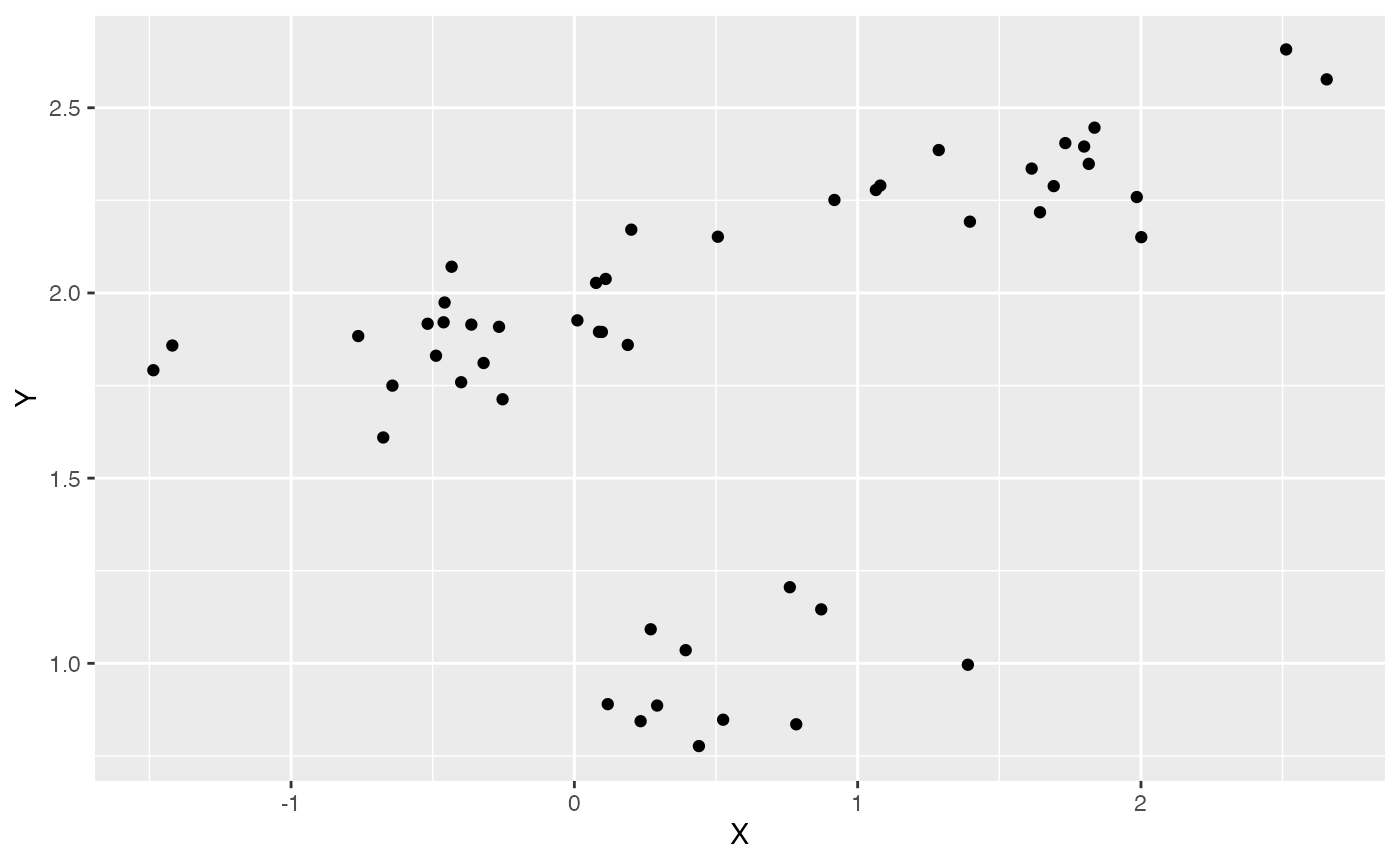

summary(lm(Y~X,df))
#> 
#> Call:
#> lm(formula = Y ~ X, data = df)
#> 
#> Residuals:
#>      Min       1Q   Median       3Q      Max 
#> -1.05210  0.02654  0.20725  0.32340  0.43378 
#> 
#> Coefficients:
#>             Estimate Std. Error t value Pr(>|t|)    
#> (Intercept)  1.73521    0.07852  22.100  < 2e-16 ***
#> X            0.19442    0.07077   2.747  0.00844 ** 
#> ---
#> Signif. codes:  0 '***' 0.001 '**' 0.01 '*' 0.05 '.' 0.1 ' ' 1
#> 
#> Residual standard error: 0.4934 on 48 degrees of freedom
#> Multiple R-squared:  0.1359, Adjusted R-squared:  0.1179 
#> F-statistic: 7.548 on 1 and 48 DF,  p-value: 0.008435

################################################################################################################

################################################################################################################
#Simulate errors 
Z_X_error<-1 #Number of X traits with error
X_error<-rep(0.01,N)
Y_error<-rep(0.01,N)
Y_with_error<-Y+rnorm(N,0,0.01)
X_with_error<-X+rnorm(N,0,0.01)


############################################################################################################
#Make trdata file
trdata$dat<-cbind(trdata$dat,data.frame(cbind(Y_with_error,Y_error,X_with_error,X_error)))

Next we will set the priors for the estimated parameters - for this model this includes the half-life, Vy, optima, and beta. For the latter two parameters we will use the results of the linear model to inform our priors.

############################################################################################################
#Set Priors
hl.prior<-c(log(0.25),0.75)
vy.prior<-5
optima.prior<-c(1.5,0.5) #Informed by linear model
beta.prior<-c(0.2,0.25) #Informed by linear model

Exploring Priors

At this point one would want to explore if the priors are appropriate - do the prior distributions look consistent with what we know about our system? See Grabowski (in press) for more on setting priors.

Half-life Prior plot

hl.sims<-data.frame(rlnorm(n=1000,meanlog=hl.prior[1],sdlog=hl.prior[2]))
names(hl.sims)<-"prior.hl.sims"

hl.prior.plot<-ggplot2::ggplot()+
  ggplot2::geom_density(ggplot2::aes(prior.hl.sims,fill="prior.hl.sims"),alpha=0.2,data=hl.sims)+
  ggplot2::theme_bw()+
  ggplot2::theme(
    panel.grid.major = ggplot2::element_blank(),
    panel.grid.minor = ggplot2::element_blank())+
  
  #labs(title="Prior vs. Posterior Distribution ",x="Half-life", y = "Density")+
  ggplot2::labs(title="",x="Half-life", y = "Density")+
  
  #scale_fill_manual(labels=c("Posterior","Prior"))+
  ggplot2::geom_vline(xintercept=c(hl),linetype=2)+
  ggsci::scale_fill_npg(name="",labels=c("Prior"))

hl.prior.plot

Vy Prior Plot

vy.sims<-rexp(n=1000,rate=vy.prior)
vy.sims<-data.frame(vy.sims)
names(vy.sims)<-"prior.vy.sims"

vy.prior.plot<-ggplot2::ggplot()+
  ggplot2::geom_density(ggplot2::aes(prior.vy.sims,fill="prior.vy.sims"),alpha=0.2,data=vy.sims)+
  ggplot2::theme_bw()+
  ggplot2::theme(
    panel.grid.major = ggplot2::element_blank(),
    panel.grid.minor = ggplot2::element_blank())+
  
  #labs(title="Prior vs. Posterior Distribution ",x="vy", y = "Density")+
  ggplot2::labs(title="",x="vy", y = "Density")+
  ggplot2::geom_vline(xintercept=c(vy),linetype=2)+
  
  #scale_fill_manual(labels=c("Posterior","Prior"))+
  ggsci::scale_fill_npg(name="",labels=c("Prior"))


vy.prior.plot

Prior on how shared branch lengths correspond to covariance

a.sims<-log(2)/hl.sims;
sigma2_y.sims<-vy.sims*(2*(log(2)/hl.sims));
beta.sims<-rnorm(n=100,beta.prior[1],beta.prior[2])

plot( NULL , xlim=c(0,1) , ylim=c(0,0.4) , xlab="Time since MRCA" , ylab="Covariance" ,cex.axis=0.75, mgp=c(1.25,0.25,0),tcl=-0.25)
for (i in 1:30){
  curve(calc_multiadaptive_cov_plot(a.sims[i,],sigma2_y.sims[i,],beta.sims[i],x) , add=TRUE , lwd=4 , col=rethinking::col.alpha(1,0.15))
}

par(mar=c(3,3,0.25,0.25))

Slope and intercept Prior Plot

optima.sims<-rnorm(100,optima.prior[1],optima.prior[2])
beta.sims<-rnorm(n=100,beta.prior[1],beta.prior[2])

prior.slope.plot<-ggplot2::ggplot()+  
 ggplot2:: geom_point(data=df,ggplot2::aes(y=Y,x=X))+
  ggplot2::geom_abline(intercept=optima.sims,slope=beta.sims,alpha=0.15)+
  ggplot2::theme_bw()+
  ggplot2::theme(
    panel.grid.major = ggplot2::element_blank(),
    panel.grid.minor = ggplot2::element_blank())+
  
  ggplot2::ylab("Y") + ggplot2::xlab("Adaptive X")+
  ggsci::scale_color_npg()

prior.slope.plot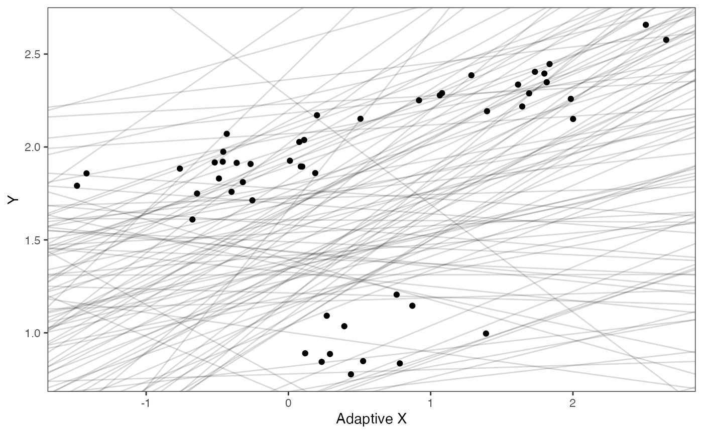

We will use the helper function blouch.reg.adapt.prep() to setup the dat file for Stan. Here “Z_adaptive” is the number of predictors, and “regimes” is the name of the regime column in trdata$dat.

############################################################################################################
#Test Blouch prep code - Regimes + Direct Efffect model
dat<-blouch.reg.adapt.prep(trdata,"Y_with_error","Y_error","X_with_error","X_error",Z_adaptive=1,"regimes",hl.prior,vy.prior,optima.prior,beta.prior)

First we will run the Multi-optima Adaptive Model with Varying Effects

fit.reg.adapt.ve<- rstan::sampling(object = blouch:::stanmodels$blouchOU_reg_adapt_ve,data = dat,chains = 2,cores=2,iter=2000)
#> Found more than one class "stanfit" in cache; using the first, from namespace 'rstan'
#> Also defined by 'rethinking'
#> Found more than one class "stanfit" in cache; using the first, from namespace 'rstan'
#> Also defined by 'rethinking'

print(fit.reg.adapt.ve,pars = c("hl","vy","optima","beta"))
#> Inference for Stan model: blouchOU_reg_adapt_ve.
#> 2 chains, each with iter=2000; warmup=1000; thin=1; 
#> post-warmup draws per chain=1000, total post-warmup draws=2000.
#> 
#>           mean se_mean   sd  2.5%  25%  50%  75% 97.5% n_eff Rhat
#> hl        0.19    0.00 0.11  0.06 0.12 0.17 0.24  0.47   708    1
#> vy        0.02    0.00 0.01  0.00 0.01 0.01 0.02  0.03  1547    1
#> optima[1] 1.99    0.00 0.06  1.88 1.96 1.99 2.02  2.10  2625    1
#> optima[2] 0.84    0.01 0.15  0.45 0.77 0.86 0.94  1.05   730    1
#> beta[1,1] 0.26    0.00 0.06  0.18 0.23 0.25 0.29  0.40   992    1
#> beta[2,1] 0.12    0.00 0.13 -0.14 0.04 0.12 0.21  0.38  2207    1
#> 
#> Samples were drawn using NUTS(diag_e) at Tue Oct  8 14:14:19 2024.
#> For each parameter, n_eff is a crude measure of effective sample size,
#> and Rhat is the potential scale reduction factor on split chains (at 
#> convergence, Rhat=1).
post<-rstan::extract(fit.reg.adapt.ve) #rstan::extract posterior distribution

Prior vs. posterior

hl.post<-data.frame(post$hl)
names(hl.post)<-"post.hl.sims"

hl.plot<-ggplot2::ggplot()+
  ggplot2::geom_density(ggplot2::aes(prior.hl.sims,fill="prior.hl.sims"),alpha=0.2,data=hl.sims)+
  ggplot2::geom_density(ggplot2::aes(post.hl.sims,fill="post.hl.sims"),alpha=0.2,data=hl.post)+
  ggplot2::theme_bw()+
  ggplot2::theme(
    panel.grid.major = ggplot2::element_blank(),
    panel.grid.minor = ggplot2::element_blank())+
  
  #labs(title="Prior vs. Posterior Distribution ",x="Half-life", y = "Density")+
  ggplot2::labs(title="",x="Half-life", y = "Density")+
  
  #scale_fill_manual(labels=c("Posterior","Prior"))+
  ggplot2::geom_vline(xintercept=c(hl),linetype=2)+
  ggsci::scale_fill_npg(name="",labels=c("Posterior","Prior"))

hl.plot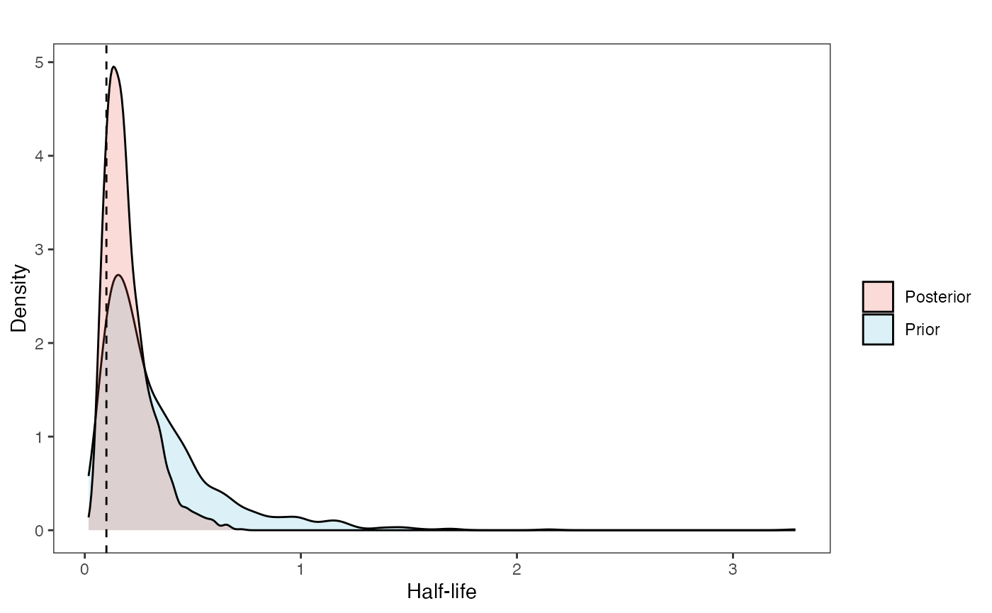

Prior vs. posterior plot

vy.post<-data.frame(post$vy)
names(vy.post)<-"post.vy.sims"

vy.plot<-ggplot2::ggplot()+
  ggplot2::geom_density(ggplot2::aes(prior.vy.sims,fill="prior.vy.sims"),alpha=0.2,data=vy.sims)+
  ggplot2::geom_density(ggplot2::aes(post.vy.sims,fill="post.vy.sims"),alpha=0.2,data=vy.post)+
  ggplot2::theme_bw()+
  ggplot2::theme(
    panel.grid.major = ggplot2::element_blank(),
    panel.grid.minor = ggplot2::element_blank())+
  
  #labs(title="Prior vs. Posterior Distribution ",x="vy", y = "Density")+
  ggplot2::labs(title="",x="vy", y = "Density")+
  ggplot2::geom_vline(xintercept=c(vy),linetype=2)+
  
  #scale_fill_manual(labels=c("Posterior","Prior"))+
  ggsci::scale_fill_npg(name="",labels=c("Posterior","Prior"))

vy.plot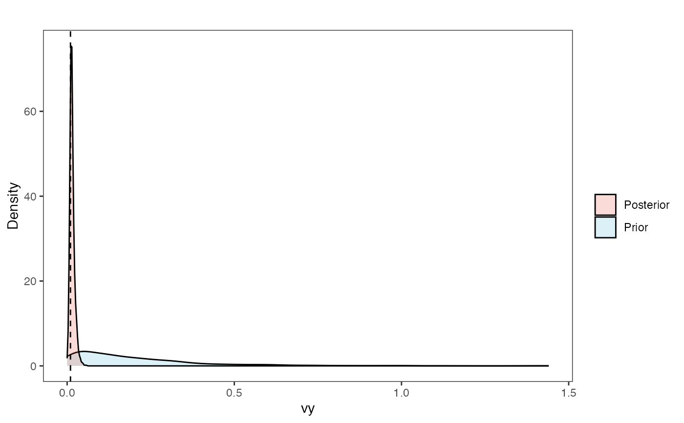

Adaptation model

a.sims<-log(2)/hl.sims;
sigma2_y.sims<-vy.sims*(2*(log(2)/hl.sims));
beta.sims<-rnorm(n=100,beta.prior[1],beta.prior[2])

plot( NULL , xlim=c(0,1) , ylim=c(0,0.3) , xlab="Time since MRCA" , ylab="Covariance" ,cex.axis=0.75, mgp=c(1.25,0.25,0),tcl=-0.25)
for (i in 1:30){
  curve(calc_multiadaptive_cov_plot(a.sims[i,],sigma2_y.sims[i,],beta.sims[i],x) , add=TRUE , lwd=4 , col=rethinking::col.alpha(1,0.15))
}

for (i in 1:30){
  curve(calc_multiadaptive_cov_plot(post$a[i],post$sigma2_y[i],as.numeric(data.frame(post$beta)[i,]),x) , add=TRUE , lwd=4 , col=rethinking::col.alpha(2,0.5))
  #curve(calc_multiadaptive_cov(post$a[i],post$sigma2_y[i],beta,x,Z_adaptive,n_reg) , add=TRUE , lwd=4 , col=col.alpha(2,0.5))
}

#multiple traits


par(mar=c(3,3,0.25,0.25))
covariance.plot <- recordPlot()
dev.off()
#> null device 
#>           1

#Vt = sigma2_y /( 2 * a) * ((1 - exp(-2 * a * ta)) .* exp(-a * tij)); //From Hansen (1997)

covariance.plot

Priors + Posteriors

optima.sims<-rnorm(100,optima.prior[1],optima.prior[2])
beta.sims<-rnorm(n=100,beta.prior[1],beta.prior[2])


optima.post<-post$optima
beta.post<-data.frame(post$beta)
names(beta.post)<-c("post.beta.1","post.beta.2")

mu.link.11<-function(x.seq){optima.post[,1]+x.seq*beta.post[,1]}
mu.link.12<-function(x.seq){optima.post[,2]+x.seq*beta.post[,2]}

x.seq <- seq(from=min(X), to=max(X) , length.out=100)
mu.11 <- sapply(x.seq , mu.link.11 )
mu.12 <- sapply(x.seq , mu.link.12 )

#mu.mean.11 <-lapply( mu.11 , mean )
#mu.mean.12 <-lapply( mu.12 , mean )

mu.mean.11<-colMeans(mu.11)
mu.mean.12<-colMeans(mu.12)

mu.mean.11<-data.frame(as.numeric(mu.mean.11))
mu.mean.12<-data.frame(as.numeric(mu.mean.12))
names(mu.mean.11)<-"mu.mean.11"
names(mu.mean.12)<-"mu.mean.12"

mu.CI.11 <- apply( mu.11 , MARGIN=2, FUN=rethinking::PI , prob=0.89 )
mu.CI.12 <- apply( mu.12 , MARGIN=2, FUN=rethinking::PI , prob=0.89 )

#mu.CI.11 <- lapply( mu.11 , PI , prob=0.89 )
#mu.CI.12 <- lapply( mu.12 , PI , prob=0.89 )
mu.CI.11<-data.frame(t(data.frame(mu.CI.11)),x.seq)
mu.CI.12<-data.frame(t(data.frame(mu.CI.12)),x.seq)

names(mu.CI.11)<-c("min.5.5","max.94.5","x.seq")
names(mu.CI.12)<-c("min.5.5","max.94.5","x.seq")

#df<-data.frame(Y=stan_sim_data$Y,X=stan_sim_data$direct_cov)
df<-data.frame(Y=dat$Y_obs,X=dat$X_obs,Regimes=regimes_tip)
df11<-data.frame(x.seq,mu.mean.11)
df12<-data.frame(x.seq,mu.mean.12)


#slope.prior.plot<-ggplot(data=reg.trdata$dat,aes(y=Sim1,x=X))+
slope.plot.1<-ggplot2::ggplot()+  
  ggplot2::geom_point(data=df,ggplot2::aes(y=Y,x=X,color=Regimes))+
  ggplot2::geom_abline(intercept=optima.sims,slope=beta.sims,alpha=0.1)+ #Prior
  ggplot2::geom_abline(intercept=optima[1],slope=beta[1],alpha=0.5,linetype=2)+
  ggplot2::geom_abline(intercept=optima[2],slope=beta[2],alpha=0.5,linetype=2)+
  ggplot2::geom_line(data=df11,ggplot2::aes(x=x.seq,y=mu.mean.11),linetype=1)+
  ggplot2::geom_ribbon(data=mu.CI.11,ggplot2::aes(x=x.seq,ymin=min.5.5,ymax=max.94.5),linetype=2,alpha=0.25)+
  ggplot2::geom_line(data=df12,ggplot2::aes(x=x.seq,y=mu.mean.12),linetype=1)+
  ggplot2::geom_ribbon(data=mu.CI.12,ggplot2::aes(x=x.seq,ymin=min.5.5,ymax=max.94.5),linetype=2,alpha=0.25)+
  
  ggplot2::theme_bw()+
  ggplot2::theme(
    panel.grid.major = ggplot2::element_blank(),
    panel.grid.minor = ggplot2::element_blank())+
  
  #ggtitle("Prior vs. Posterior for Intercept and Slope")+
  ggplot2::ylab("Y") + ggplot2::xlab("Adaptive trait")+
  ggsci::scale_color_npg()

slope.plot.1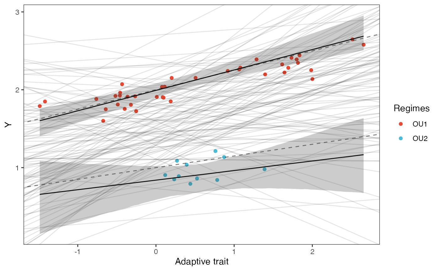

Multilevel Multi-optima Adaptive Model with Varying Effects Next we will set the priors for the estimated parameters - for this model this includes the half-life, Vy, optima, and beta. For the latter two parameters we will use the results of the linear model to inform our priors.

############################################################################################################
#Set Priors
hl.prior<-c(log(0.25),0.75)
vy.prior<-5
optima.prior<-c(1.5,0.5) #Informed by linear model
beta.prior<-c(0.2,0.25) #Informed by linear model
sigma.prior<-c(0,1)

We will use the helper function blouch.reg.adapt.prep() to setup the dat file for Stan. Here “Z_adaptive” is the number of predictors, and “regimes” is the name of the regime column in trdata$dat.

############################################################################################################
#Test Blouch prep code - Regimes + Direct Efffect model
dat<-blouch.reg.adapt.mlm.prep(trdata,"Y_with_error","Y_error","X_with_error","X_error",Z_adaptive=1,"regimes",hl.prior,vy.prior,optima.prior,beta.prior,sigma.prior)

Now we run the Multilevel Multi-optima Adaptive Model with Varying Effects, look at the results, and rstan::extract the posterior

fit.reg.adapt.mlm.ve<- rstan::sampling(object = blouch:::stanmodels$blouchOU_reg_adapt_mlm_ve,data = dat,chains = 2,cores=2,iter=2000)
#> Found more than one class "stanfit" in cache; using the first, from namespace 'rstan'
#> Also defined by 'rethinking'
#> Found more than one class "stanfit" in cache; using the first, from namespace 'rstan'
#> Also defined by 'rethinking'
#> Warning: There were 101 divergent transitions after warmup. See
#> https://mc-stan.org/misc/warnings.html#divergent-transitions-after-warmup
#> to find out why this is a problem and how to eliminate them.
#> Warning: Examine the pairs() plot to diagnose sampling problems

print(fit.reg.adapt.mlm.ve,pars = c("hl","vy","optima","beta","sigma","optima_bar","beta_bar","Rho"))
#> Inference for Stan model: blouchOU_reg_adapt_mlm_ve.
#> 2 chains, each with iter=2000; warmup=1000; thin=1; 
#> post-warmup draws per chain=1000, total post-warmup draws=2000.
#> 
#>             mean se_mean   sd  2.5%   25%  50%  75% 97.5% n_eff Rhat
#> hl          0.23    0.01 0.15  0.07  0.13 0.19 0.29  0.63   386 1.01
#> vy          0.02    0.00 0.01  0.00  0.01 0.01 0.02  0.04   771 1.00
#> optima[1]   2.00    0.00 0.06  1.88  1.96 2.00 2.04  2.13  1327 1.00
#> optima[2]   0.77    0.01 0.23  0.15  0.70 0.83 0.91  1.04   367 1.01
#> beta[1,1]   0.28    0.00 0.08  0.18  0.23 0.26 0.31  0.48   376 1.01
#> beta[2,1]   0.16    0.01 0.16 -0.16  0.06 0.17 0.27  0.48   701 1.00
#> sigma[1]    0.95    0.01 0.44  0.37  0.62 0.87 1.19  2.01  1508 1.00
#> sigma[2]    0.32    0.01 0.32  0.03  0.10 0.21 0.44  1.25  1273 1.00
#> optima_bar  1.47    0.01 0.40  0.71  1.20 1.46 1.72  2.24  1611 1.00
#> beta_bar[1] 0.22    0.01 0.16 -0.13  0.13 0.23 0.31  0.54   787 1.00
#> Rho[1,1]    1.00     NaN 0.00  1.00  1.00 1.00 1.00  1.00   NaN  NaN
#> Rho[1,2]    0.08    0.01 0.43 -0.73 -0.25 0.09 0.40  0.84  1723 1.00
#> Rho[2,1]    0.08    0.01 0.43 -0.73 -0.25 0.09 0.40  0.84  1723 1.00
#> Rho[2,2]    1.00    0.00 0.00  1.00  1.00 1.00 1.00  1.00  2030 1.00
#> 
#> Samples were drawn using NUTS(diag_e) at Tue Oct  8 14:15:11 2024.
#> For each parameter, n_eff is a crude measure of effective sample size,
#> and Rhat is the potential scale reduction factor on split chains (at 
#> convergence, Rhat=1).
post<-rstan::extract(fit.reg.adapt.mlm.ve) #rstan::extract posterior distribution

Now we run the non-centered version of the Multilevel Multi-optima Adaptive Model with Varying Effects

fit.reg.adapt.mlm.ve.nc<- rstan::sampling(object = blouch:::stanmodels$blouchOU_reg_adapt_mlm_ve_nc,data = dat,chains = 2,cores=2,iter=2000)
#> Found more than one class "stanfit" in cache; using the first, from namespace 'rstan'
#> Also defined by 'rethinking'
#> Found more than one class "stanfit" in cache; using the first, from namespace 'rstan'
#> Also defined by 'rethinking'
#> Warning: There were 16 divergent transitions after warmup. See
#> https://mc-stan.org/misc/warnings.html#divergent-transitions-after-warmup
#> to find out why this is a problem and how to eliminate them.
#> Warning: Examine the pairs() plot to diagnose sampling problems

print(fit.reg.adapt.mlm.ve,pars = c("hl","vy","optima","beta","sigma","optima_bar","beta_bar","Rho"))
#> Inference for Stan model: blouchOU_reg_adapt_mlm_ve.
#> 2 chains, each with iter=2000; warmup=1000; thin=1; 
#> post-warmup draws per chain=1000, total post-warmup draws=2000.
#> 
#>             mean se_mean   sd  2.5%   25%  50%  75% 97.5% n_eff Rhat
#> hl          0.23    0.01 0.15  0.07  0.13 0.19 0.29  0.63   386 1.01
#> vy          0.02    0.00 0.01  0.00  0.01 0.01 0.02  0.04   771 1.00
#> optima[1]   2.00    0.00 0.06  1.88  1.96 2.00 2.04  2.13  1327 1.00
#> optima[2]   0.77    0.01 0.23  0.15  0.70 0.83 0.91  1.04   367 1.01
#> beta[1,1]   0.28    0.00 0.08  0.18  0.23 0.26 0.31  0.48   376 1.01
#> beta[2,1]   0.16    0.01 0.16 -0.16  0.06 0.17 0.27  0.48   701 1.00
#> sigma[1]    0.95    0.01 0.44  0.37  0.62 0.87 1.19  2.01  1508 1.00
#> sigma[2]    0.32    0.01 0.32  0.03  0.10 0.21 0.44  1.25  1273 1.00
#> optima_bar  1.47    0.01 0.40  0.71  1.20 1.46 1.72  2.24  1611 1.00
#> beta_bar[1] 0.22    0.01 0.16 -0.13  0.13 0.23 0.31  0.54   787 1.00
#> Rho[1,1]    1.00     NaN 0.00  1.00  1.00 1.00 1.00  1.00   NaN  NaN
#> Rho[1,2]    0.08    0.01 0.43 -0.73 -0.25 0.09 0.40  0.84  1723 1.00
#> Rho[2,1]    0.08    0.01 0.43 -0.73 -0.25 0.09 0.40  0.84  1723 1.00
#> Rho[2,2]    1.00    0.00 0.00  1.00  1.00 1.00 1.00  1.00  2030 1.00
#> 
#> Samples were drawn using NUTS(diag_e) at Tue Oct  8 14:15:11 2024.
#> For each parameter, n_eff is a crude measure of effective sample size,
#> and Rhat is the potential scale reduction factor on split chains (at 
#> convergence, Rhat=1).
post<-rstan::extract(fit.reg.adapt.mlm.ve) #rstan::extract posterior distribution

From there the posteriors should be explored, compared to the priors, etc. following the format above

rm(list=ls())

Multi-optima Direct Effect and Adaptive models with Varying Effects - Multiple predictors

Two regimes with 1 direct and 1 adaptive trait and two slopes per regime per trait

########################################################################################################
set.seed(10)

N<-50 #Number of species
#set.seed(1) #Set seed to get same random species each time

phy <- ape::keep.tip(tree.10K,sample(tree.10K$tip.label)[1:N]) 
phy<-ape::multi2di(phy)

l.tree<-max(ape::branching.times(phy)) ## rescale tree to height 1
phy$edge.length<-phy$edge.length/l.tree 

#Set regimes - manually - 2 regimes
#Locate nodes
plot(phy,no.margin=TRUE,edge.width=2,cex=0.7)
ape::nodelabels(frame="none",adj=c(1.1,-0.4))
ape::tiplabels()

#Paint Regimes on Tree
shifts<-c(84) #Location of nodes with regime shifts
trdata<-data.frame(phy$tip.label)
trdata<-treeplyr::make.treedata(phy,trdata)
trdata<-set.converge.regimes(trdata,shifts)
#> [1] 1
#>  [1] OU1 OU1 OU1 OU1 OU1 OU1 OU1 OU1 OU1 OU1 OU1 OU1 OU1 OU1 OU1 OU1 OU1 OU1 OU1
#> [20] OU1 OU1 OU1 OU1 OU1 OU1 OU1 OU1 OU1 OU1 OU1 OU1 OU1 OU1 OU1 OU1 OU1 OU1 OU1
#> [39] OU1 OU1 OU1 OU1 OU1 OU1 OU1 OU1 OU1 OU1 OU1 OU1 OU1 OU1 OU1 OU1 OU1 OU1 OU1
#> [58] OU1 OU1 OU1 OU1 OU1 OU1 OU1 OU2 OU2 OU2 OU2 OU2 OU2 OU2 OU2 OU2 OU2 OU2 OU2
#> [77] OU2 OU2 OU2 OU2 OU2 OU2 OU2 OU2 OU2 OU1 OU1 OU1 OU1 OU1 OU1 OU1 OU1 OU1 OU1
#> [96] OU1 OU1 OU1
#> Levels: OU1 OU2
#> [1] "#E64B35FF" "#4DBBD5FF"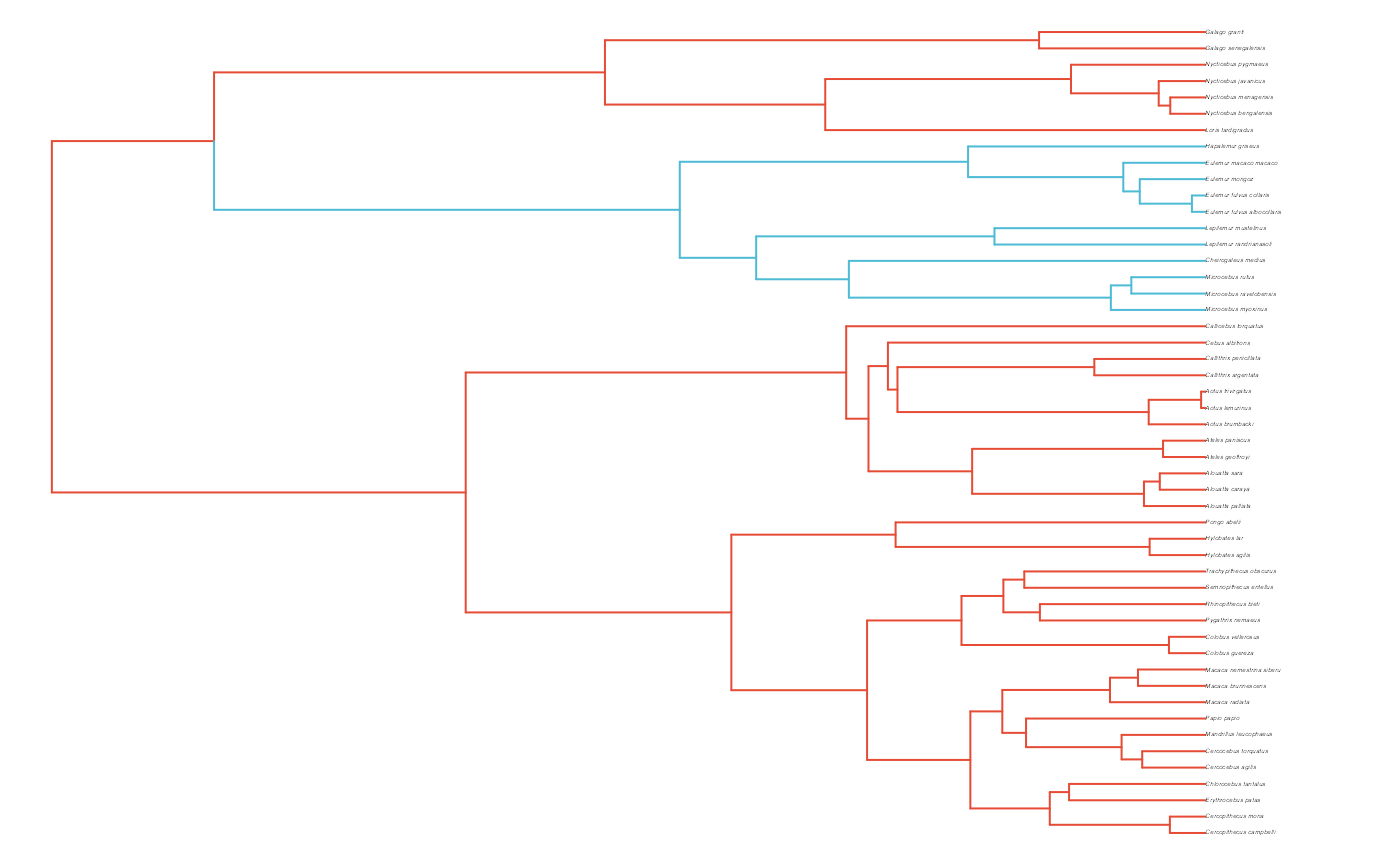

#Check if manual setting code worked
shifts.total<-c(trdata$dat$regimes,trdata$phy$node.label)
edge.regimes <- factor(shifts.total[trdata$phy$edge[,2]])
print(edge.regimes)
#>  [1] OU1 OU1 OU1 OU1 OU1 OU1 OU1 OU1 OU1 OU1 OU1 OU1 OU1 OU1 OU1 OU1 OU1 OU1 OU1
#> [20] OU1 OU1 OU1 OU1 OU1 OU1 OU1 OU1 OU1 OU1 OU1 OU1 OU1 OU1 OU1 OU1 OU1 OU1 OU1
#> [39] OU1 OU1 OU1 OU1 OU1 OU1 OU1 OU1 OU1 OU1 OU1 OU1 OU1 OU1 OU1 OU1 OU1 OU1 OU1
#> [58] OU1 OU1 OU1 OU1 OU1 OU1 OU1 OU2 OU2 OU2 OU2 OU2 OU2 OU2 OU2 OU2 OU2 OU2 OU2
#> [77] OU2 OU2 OU2 OU2 OU2 OU2 OU2 OU2 OU2 OU1 OU1 OU1 OU1 OU1 OU1 OU1 OU1 OU1 OU1
#> [96] OU1 OU1 OU1
#> Levels: OU1 OU2

reg_tips<-trdata$dat$regimes
reg_tips<-as.numeric(as.factor(reg_tips))

reg.colors <- ggsci::pal_aaas("default", alpha = 0.7)(2)
print(reg.colors)
#> [1] "#3B4992B2" "#EE0000B2"
plot(trdata$phy,edge.color = reg.colors[edge.regimes], edge.width = 1, cex = 0.2)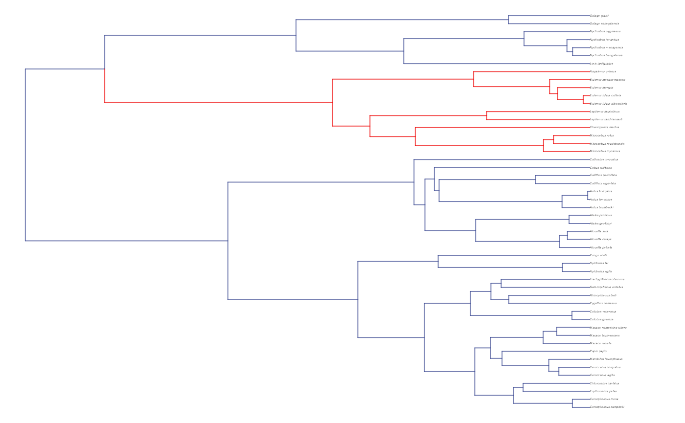

#Phylogeny info
n<-length(trdata$phy$tip.label)

regimes_internal <-trdata$phy$node.label
regimes_tip <- trdata$dat$regimes
regimes <- concat.factor(regimes_tip, regimes_internal)
anc_maps<-"regimes"
lineages <- lapply(1:n, function(e) lineage.constructor(phy, e, anc_maps, regimes)) #Trace lineage from tips (n) to root and determine regimes of each node or branch

Simulate X and Y data using generative model

################################################################################################################
hl<-0.1 #0.1, 0.25, 0.75 - testing options
a<-log(2)/hl
vy<-0.01 #0.25,0.5 - testing options
sigma2_y<-vy*(2*(log(2)/hl));

vX0<-0
vY0 <- 0
sigma2_x<-matrix(10,1,1) #Variance of BM Process

Xa<-phytools::fastBM(phy,a=vX0,sig2=sigma2_x[1,1],internal=FALSE) #Simulate X BM variable on tree, with scaling 10
Xd<-phytools::fastBM(phy,a=vX0,sig2=sigma2_x[1,1],internal=FALSE) #Simulate X BM variable on tree, with scaling 10

names(Xa)<-phy$tip.label
names(Xd)<-phy$tip.label
phytools::phenogram(phy,Xd,spread.labels=TRUE,spread.cost=c(1,0)) #Plot X data
#> Optimizing the positions of the tip labels...

phytools::phenogram(phy,Xa,spread.labels=TRUE,spread.cost=c(1,0)) #Plot X data
#> Optimizing the positions of the tip labels...

Xs<-cbind(Xd,Xa)

Z_adaptive<-1
Z_direct<-1

optima_matrix<-weight.matrix(phy, a, lineages) #Slouch approach
pred_X<-calc_mixed_dmX(phy,a,Xs,Z_direct,Z_adaptive)
optima<-c(2,1.5)
beta<-data.frame(matrix(c(0.25,0.15,0.35,0.1),ncol=2,nrow=2)) #Direct efect - column 1, Adaptive, column 2, slopes for regimes on rows

mu<-matrix(NA,N,1)
for(i in 1:N){
  mu[i] = optima_matrix[i,]%*%optima+pred_X[i,]%*%t(beta[reg_tips[i],])
  }

n_reg<-length(unique(regimes))
V<-calc_adaptive_V(phy,a, sigma2_y, beta[,2],  sigma2_x, Z_adaptive)
Y<-MASS::mvrnorm(n=1,mu,V)


###############################################################################################################

summary(lm(Y~Xs))
#> 
#> Call:
#> lm(formula = Y ~ Xs)
#> 
#> Residuals:
#>      Min       1Q   Median       3Q      Max 
#> -0.72841 -0.19574 -0.01492  0.22366  0.85254 
#> 
#> Coefficients:
#>             Estimate Std. Error t value Pr(>|t|)    
#> (Intercept)  1.80422    0.07225   24.97   <2e-16 ***
#> XsXd         0.26776    0.01919   13.95   <2e-16 ***
#> XsXa         0.30498    0.01524   20.01   <2e-16 ***
#> ---
#> Signif. codes:  0 '***' 0.001 '**' 0.01 '*' 0.05 '.' 0.1 ' ' 1
#> 
#> Residual standard error: 0.313 on 47 degrees of freedom
#> Multiple R-squared:  0.9514, Adjusted R-squared:  0.9494 
#> F-statistic: 460.4 on 2 and 47 DF,  p-value: < 2.2e-16

################################################################################################################

###############################################################################################################
#Simulate errors - original Hansen setup
Z_X_error<-2 #Number of X traits with error
X_error<-matrix(0.01,nrow=N,ncol=Z_X_error)
X_error<-data.frame(X_error)
names(X_error)<-c("Xd_error","Xa_error")
Y_error<-rep(0.01,N)
Y_with_error<-Y+rnorm(N,0,0.01)
X_with_error<-Xs+rnorm(N,0,0.01)
X_with_error<-data.frame(X_with_error)
names(X_with_error)<-c("Xd","Xa")
############################################################################################################
#Make trdata file
trdata$dat<-cbind(trdata$dat,data.frame(cbind(Y_with_error,Y_error,X_with_error,X_error)))
#names(trdata$dat)[6:7]<-c("Xd_error","Xa_error")

Plot Data

#Plot of data
df<-data.frame(Y=trdata$dat$Y_with_error,Xd=trdata$dat$Xd,Xa=trdata$dat$Xa,Regimes=trdata$dat$regimes)


#slope.prior.plot<-ggplot(data=reg.trdata$dat,aes(y=Sim1,x=X))+
slope.plot.1<-ggplot2::ggplot()+  
  ggplot2::geom_point(data=df,ggplot2::aes(y=Y,x=Xd,color=Regimes))+
  
  ggplot2::geom_abline(intercept=optima[1],slope=beta[1,1],alpha=0.5,linetype=2)+
  ggplot2::geom_abline(intercept=optima[2],slope=beta[2,1],alpha=0.5,linetype=2)+
  
  
  ggplot2::theme_bw()+
  ggplot2::theme(
    panel.grid.major = ggplot2::element_blank(),
    panel.grid.minor = ggplot2::element_blank())+
  
  #ggtitle("Prior vs. Posterior for Intercept and Slope")+
  ggplot2::ylab("Y") + ggplot2::xlab("Direct effect trait")+
  ggsci::scale_color_npg()

slope.plot.1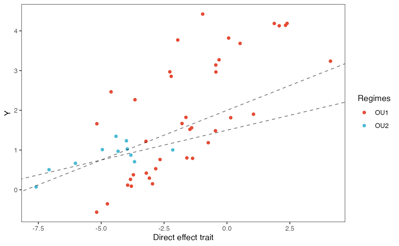

#slope.prior.plot<-ggplot(data=reg.trdata$dat,aes(y=Sim1,x=X))+
slope.plot.2<-ggplot2::ggplot()+  
  ggplot2::geom_point(data=df,ggplot2::aes(y=Y,x=Xa,color=Regimes))+
  
  ggplot2::geom_abline(intercept=optima[1],slope=beta[1,2],alpha=0.5,linetype=2)+
  ggplot2::geom_abline(intercept=optima[2],slope=beta[2,2],alpha=0.5,linetype=2)+
  
  ggplot2::theme_bw()+
  ggplot2::theme(
    panel.grid.major = ggplot2::element_blank(),
    panel.grid.minor = ggplot2::element_blank())+
  
  #ggtitle("Prior vs. Posterior for Intercept and Slope")+
  ggplot2::ylab("Y") + ggplot2::xlab("Adaptive trait")+
  ggsci::scale_color_npg()

slope.plot.2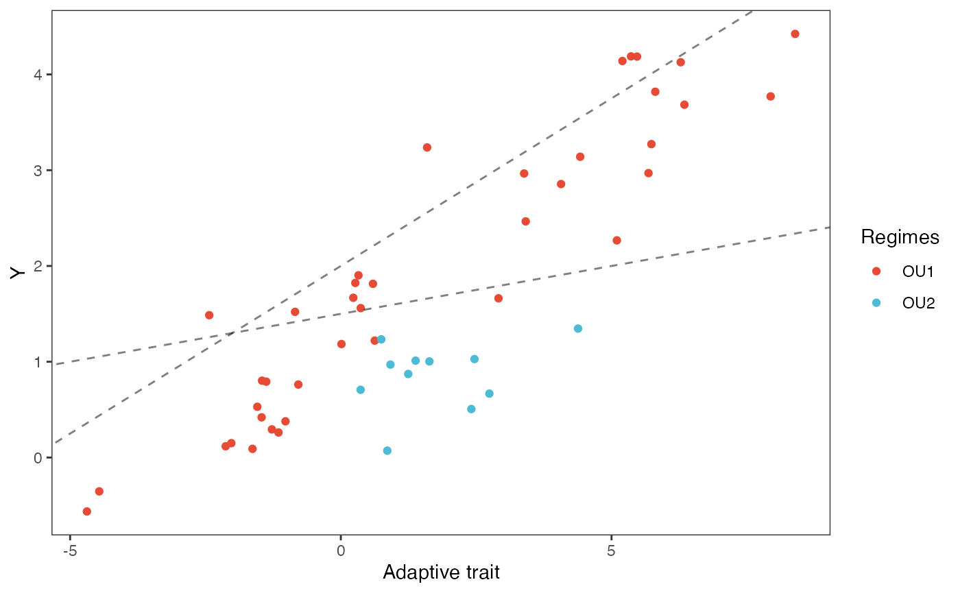

Next we will set the priors for the estimated parameters - for this model this includes the half-life, Vy, optima, and beta. For the latter two parameters we will use the results of the linear model to inform our priors.

############################################################################################################
#Set Priors
hl.prior<-c(log(0.25),0.75)
vy.prior<-20
optima.prior<-c(1.5,0.25) #Informed by linear model
beta.prior<-c(0,0.25) #Informed by linear model

Exploring Priors

At this point one would want to explore if the priors are appropriate - do the prior distributions look consistent with what we know about our system? See Grabowski (in press) for more on setting priors.

Half-life Prior plot

hl.sims<-data.frame(rlnorm(n=1000,meanlog=hl.prior[1],sdlog=hl.prior[2]))
names(hl.sims)<-"prior.hl.sims"

hl.prior.plot<-ggplot2::ggplot()+
  ggplot2::geom_density(ggplot2::aes(prior.hl.sims,fill="prior.hl.sims"),alpha=0.2,data=hl.sims)+
  ggplot2::theme_bw()+
  ggplot2::theme(
    panel.grid.major = ggplot2::element_blank(),
    panel.grid.minor = ggplot2::element_blank())+
  
  #labs(title="Prior vs. Posterior Distribution ",x="Half-life", y = "Density")+
  ggplot2::labs(title="",x="Half-life", y = "Density")+
  
  #scale_fill_manual(labels=c("Posterior","Prior"))+
  ggplot2::geom_vline(xintercept=c(hl),linetype=2)+
  ggsci::scale_fill_npg(name="",labels=c("Prior"))

hl.prior.plot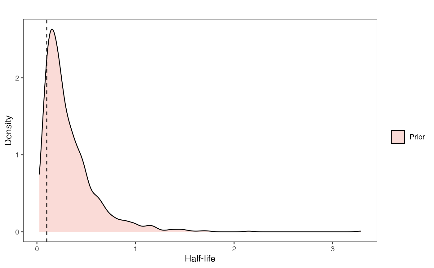

Vy Prior Plot

vy.sims<-rexp(n=1000,rate=vy.prior)
vy.sims<-data.frame(vy.sims)
names(vy.sims)<-"prior.vy.sims"

vy.prior.plot<-ggplot2::ggplot()+
  ggplot2::geom_density(ggplot2::aes(prior.vy.sims,fill="prior.vy.sims"),alpha=0.2,data=vy.sims)+
  ggplot2::theme_bw()+
  ggplot2::theme(
    panel.grid.major = ggplot2::element_blank(),
    panel.grid.minor = ggplot2::element_blank())+
  
  #labs(title="Prior vs. Posterior Distribution ",x="vy", y = "Density")+
  ggplot2::labs(title="",x="vy", y = "Density")+
  ggplot2::geom_vline(xintercept=c(vy),linetype=2)+
  
  #scale_fill_manual(labels=c("Posterior","Prior"))+
  ggsci::scale_fill_npg(name="",labels=c("Prior"))


vy.prior.plot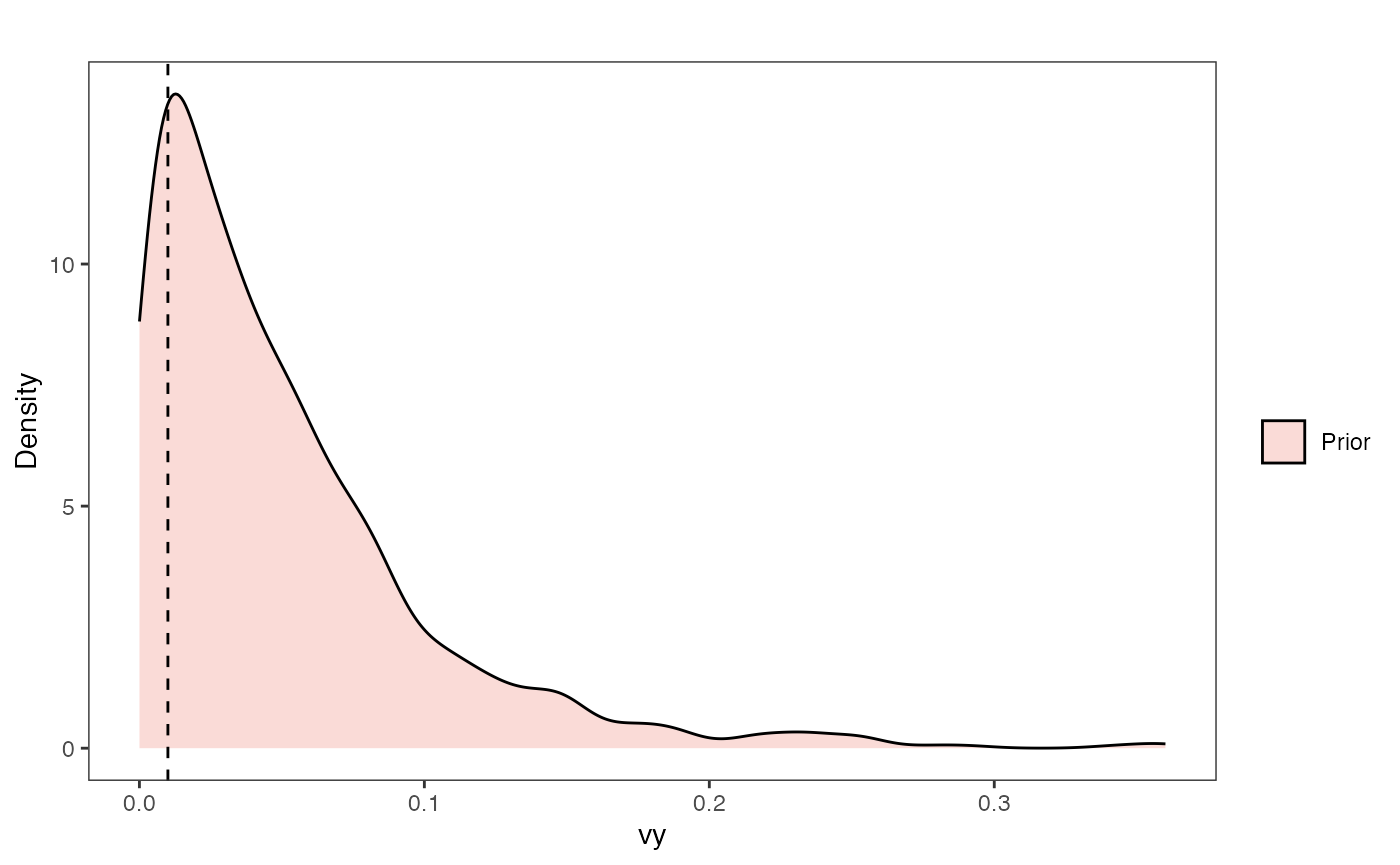

Prior on how shared branch lengths correspond to covariance

a.sims<-log(2)/hl.sims;
sigma2_y.sims<-vy.sims*(2*(log(2)/hl.sims));
beta.sims<-rnorm(n=100,beta.prior[1],beta.prior[2])

plot( NULL , xlim=c(0,1) , ylim=c(0,0.4) , xlab="Time since MRCA" , ylab="Covariance" ,cex.axis=0.75, mgp=c(1.25,0.25,0),tcl=-0.25)
for (i in 1:30){
  curve(calc_multiadaptive_cov_plot(a.sims[i,],sigma2_y.sims[i,],beta.sims[i],x) , add=TRUE , lwd=4 , col=rethinking::col.alpha(1,0.15))
}

par(mar=c(3,3,0.25,0.25))

Slope and intercept Prior Plot

optima.sims<-rnorm(100,optima.prior[1],optima.prior[2])
beta.sims<-rnorm(n=100,beta.prior[1],beta.prior[2])

prior.slope.plot<-ggplot2::ggplot()+  
 ggplot2:: geom_point(data=df,ggplot2::aes(y=Y,x=Xd))+
  ggplot2::geom_abline(intercept=optima.sims,slope=beta.sims,alpha=0.15)+
  ggplot2::theme_bw()+
  ggplot2::theme(
    panel.grid.major = ggplot2::element_blank(),
    panel.grid.minor = ggplot2::element_blank())+
  
  ggplot2::ylab("Y") + ggplot2::xlab("Direct Effect X")+
  ggsci::scale_color_npg()

prior.slope.plot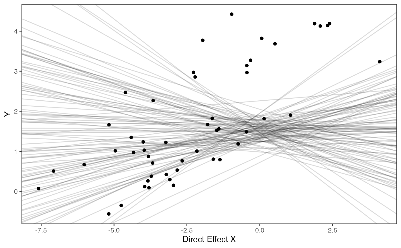

prior.slope.plot<-ggplot2::ggplot()+  
 ggplot2:: geom_point(data=df,ggplot2::aes(y=Y,x=Xa))+
  ggplot2::geom_abline(intercept=optima.sims,slope=beta.sims,alpha=0.15)+
  ggplot2::theme_bw()+
  ggplot2::theme(
    panel.grid.major = ggplot2::element_blank(),
    panel.grid.minor = ggplot2::element_blank())+
  
  ggplot2::ylab("Y") + ggplot2::xlab("Adaptive X")+
  ggsci::scale_color_npg()

prior.slope.plot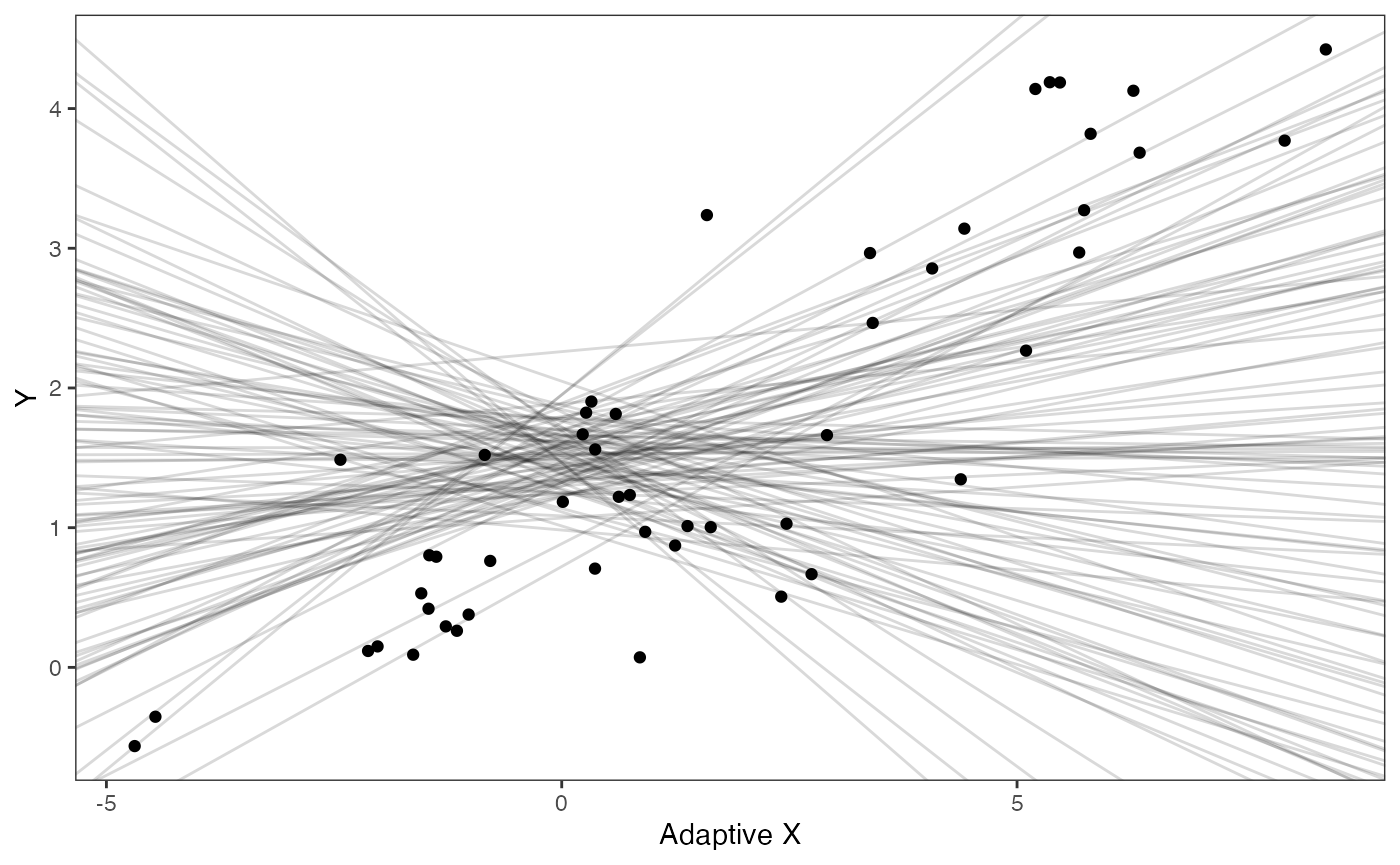

We will use the helper function blouch.reg.adapt.prep() to setup the dat file for Stan. Here “Z_adaptive” is the number of predictors, and “regimes” is the name of the regime column in trdata$dat.

############################################################################################################
dat<-blouch.reg.direct.adapt.prep(trdata,"Y_with_error","Y_error",c("Xd","Xa"),c("Xd_error","Xa_error"),Z_direct=1,Z_adaptive=1,"regimes",hl.prior,vy.prior,optima.prior,beta.prior)

First we run the Multi-optima Direct Effect Adaptive Model with Varying Effects

fit.reg.direct.adapt.ve<- rstan::sampling(object = blouch:::stanmodels$blouchOU_reg_direct_adapt_ve,data = dat,chains = 2,cores=2,iter=2000)
#> Found more than one class "stanfit" in cache; using the first, from namespace 'rstan'
#> Also defined by 'rethinking'
#> Found more than one class "stanfit" in cache; using the first, from namespace 'rstan'
#> Also defined by 'rethinking'

Let’s look at the results

print(fit.reg.direct.adapt.ve,pars = c("hl","vy","optima","beta"))
#> Inference for Stan model: blouchOU_reg_direct_adapt_ve.
#> 2 chains, each with iter=2000; warmup=1000; thin=1; 
#> post-warmup draws per chain=1000, total post-warmup draws=2000.
#> 
#>           mean se_mean   sd  2.5%  25%  50%  75% 97.5% n_eff Rhat
#> hl        0.12       0 0.07  0.05 0.08 0.10 0.14  0.32   338 1.01
#> vy        0.01       0 0.01  0.00 0.00 0.01 0.02  0.05  2698 1.00
#> optima[1] 1.70       0 0.12  1.45 1.62 1.70 1.78  1.94  3302 1.00
#> optima[2] 1.46       0 0.20  1.05 1.33 1.47 1.60  1.87  3154 1.00
#> beta[1,1] 0.22       0 0.03  0.17 0.20 0.22 0.24  0.27  4365 1.00
#> beta[1,2] 0.38       0 0.05  0.32 0.35 0.37 0.39  0.48   329 1.01
#> beta[2,1] 0.16       0 0.05  0.06 0.13 0.16 0.19  0.26  3150 1.00
#> beta[2,2] 0.10       0 0.07 -0.05 0.05 0.10 0.15  0.25  4100 1.00
#> 
#> Samples were drawn using NUTS(diag_e) at Tue Oct  8 14:17:30 2024.
#> For each parameter, n_eff is a crude measure of effective sample size,
#> and Rhat is the potential scale reduction factor on split chains (at 
#> convergence, Rhat=1).
post<-rstan::extract(fit.reg.direct.adapt.ve)

Rember, the true values are optima<-c(2,1) beta<-data.frame(matrix(c(0.25,0.15,0.35,0.1),ncol=2,nrow=2)) Direct effect - column 1, Adaptive, column 2, rows - slopes for regimes

Prior vs. posterior

hl.post<-data.frame(post$hl)
names(hl.post)<-"post.hl.sims"

hl.plot<-ggplot2::ggplot()+
  ggplot2::geom_density(ggplot2::aes(prior.hl.sims,fill="prior.hl.sims"),alpha=0.2,data=hl.sims)+
  ggplot2::geom_density(ggplot2::aes(post.hl.sims,fill="post.hl.sims"),alpha=0.2,data=hl.post)+
  ggplot2::theme_bw()+
  ggplot2::theme(
    panel.grid.major = ggplot2::element_blank(),
    panel.grid.minor = ggplot2::element_blank())+
  
  #labs(title="Prior vs. Posterior Distribution ",x="Half-life", y = "Density")+
  ggplot2::labs(title="",x="Half-life", y = "Density")+
  
  #scale_fill_manual(labels=c("Posterior","Prior"))+
  ggplot2::geom_vline(xintercept=c(hl),linetype=2)+
  ggsci::scale_fill_npg(name="",labels=c("Posterior","Prior"))

hl.plot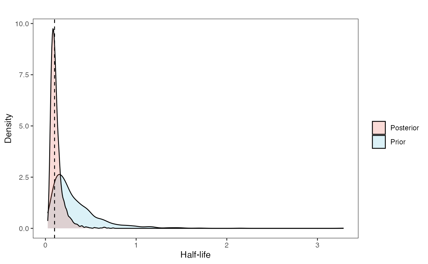

Prior vs. posterior plot

vy.post<-data.frame(post$vy)
names(vy.post)<-"post.vy.sims"

vy.plot<-ggplot2::ggplot()+
  ggplot2::geom_density(ggplot2::aes(prior.vy.sims,fill="prior.vy.sims"),alpha=0.2,data=vy.sims)+
  ggplot2::geom_density(ggplot2::aes(post.vy.sims,fill="post.vy.sims"),alpha=0.2,data=vy.post)+
  ggplot2::theme_bw()+
  ggplot2::theme(
    panel.grid.major = ggplot2::element_blank(),
    panel.grid.minor = ggplot2::element_blank())+
  
  #labs(title="Prior vs. Posterior Distribution ",x="vy", y = "Density")+
  ggplot2::labs(title="",x="vy", y = "Density")+
  ggplot2::geom_vline(xintercept=c(vy),linetype=2)+
  
  #scale_fill_manual(labels=c("Posterior","Prior"))+
  ggsci::scale_fill_npg(name="",labels=c("Posterior","Prior"))

vy.plot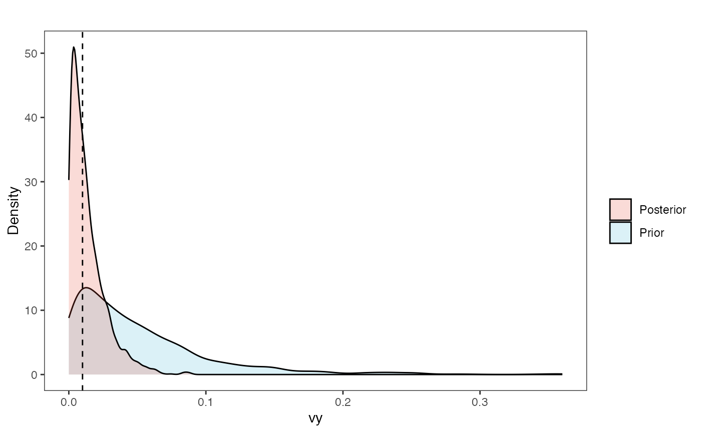

Adaptation model

a.sims<-log(2)/hl.sims;
sigma2_y.sims<-vy.sims*(2*(log(2)/hl.sims));
beta.sims<-rnorm(n=100,beta.prior[1],beta.prior[2])

plot( NULL , xlim=c(0,1) , ylim=c(0,0.3) , xlab="Time since MRCA" , ylab="Covariance" ,cex.axis=0.75, mgp=c(1.25,0.25,0),tcl=-0.25)
for (i in 1:30){
  curve(calc_multiadaptive_cov_plot(a.sims[i,],sigma2_y.sims[i,],beta.sims[i],x) , add=TRUE , lwd=4 ,
  #curve(calc_multiadaptive_cov_plot(a.sims[i,],sigma2_y.sims[i,],beta.sims[i,],x) , add=TRUE , lwd=4 ,
        col=rethinking::col.alpha(1,0.15))
}

for (i in 1:30){
  curve(calc_multiadaptive_cov_plot(post$a[i],post$sigma2_y[i],as.numeric(data.frame(post$beta)[i,,2]),x) , add=TRUE , lwd=4 , col=rethinking::col.alpha(2,0.5))
  #curve(calc_multiadaptive_cov(post$a[i],post$sigma2_y[i],beta,x,Z_adaptive,n_reg) , add=TRUE , lwd=4 , col=col.alpha(2,0.5))
}

#multiple traits


par(mar=c(3,3,0.25,0.25))
covariance.plot <- recordPlot()
dev.off()
#> null device 
#>           1

#Vt = sigma2_y /( 2 * a) * ((1 - exp(-2 * a * ta)) .* exp(-a * tij)); //From Hansen (1997)

covariance.plot

Now lets plot the prior vs. posterior plots

optima.post<-post$optima
beta.post.Xd<-data.frame(post$beta[,,1])
beta.post.Xa<-data.frame(post$beta[,,2])
names(beta.post.Xd)<-c("post.beta.1","post.beta.2")
names(beta.post.Xa)<-c("post.beta.1","post.beta.2")

mu.link.Xd1<-function(x.seq){optima.post[,1]+x.seq*beta.post.Xd[,1]}
mu.link.Xd2<-function(x.seq){optima.post[,2]+x.seq*beta.post.Xd[,2]}

x.seq <- seq(from=min(dat$X_obs[,1]), to=max(dat$X_obs[,1]) , length.out=100)
mu.11 <- sapply(x.seq , mu.link.Xd1 )
mu.12 <- sapply(x.seq , mu.link.Xd2 )

mu.mean.11<-colMeans(mu.11)
mu.mean.12<-colMeans(mu.12)

mu.mean.11<-data.frame(as.numeric(mu.mean.11))
mu.mean.12<-data.frame(as.numeric(mu.mean.12))
names(mu.mean.11)<-"mu.mean.11"
names(mu.mean.12)<-"mu.mean.12"

mu.CI.11 <- apply( mu.11 , MARGIN=2, FUN=rethinking::PI , prob=0.89 )
mu.CI.12 <- apply( mu.12 , MARGIN=2, FUN=rethinking::PI , prob=0.89 )

mu.CI.11<-data.frame(t(data.frame(mu.CI.11)),x.seq)
mu.CI.12<-data.frame(t(data.frame(mu.CI.12)),x.seq)

names(mu.CI.11)<-c("min.5.5","max.94.5","x.seq")
names(mu.CI.12)<-c("min.5.5","max.94.5","x.seq")

df<-data.frame(Y=dat$Y_obs,X=dat$X_obs,Regimes=regimes_tip)
df11<-data.frame(x.seq,mu.mean.11)
df12<-data.frame(x.seq,mu.mean.12)

mypal <- ggsci::pal_npg("nrc", alpha = 0.7)(length(beta))

slope.plot.1<-ggplot2::ggplot()+  
  ggplot2::geom_point(data=df,ggplot2::aes(y=Y,x=X.Xd,color=Regimes))+
  ggplot2::geom_abline(intercept=optima.sims,slope=beta.sims,alpha=0.15)+ #Prior
  ggplot2::geom_line(data=df11,ggplot2::aes(x=x.seq,y=mu.mean.11),linetype=1)+
  ggplot2::geom_abline(intercept=optima[1],slope=beta[1,1],alpha=0.5,linetype=2)+
  ggplot2::geom_abline(intercept=optima[2],slope=beta[2,1],alpha=0.5,linetype=2)+
  
  ggplot2::geom_ribbon(data=mu.CI.11,ggplot2::aes(x=x.seq,ymin=min.5.5,ymax=max.94.5),linetype=2,alpha=0.25)+
  ggplot2::geom_line(data=df12,ggplot2::aes(x=x.seq,y=mu.mean.12),linetype=1)+
  ggplot2::geom_ribbon(data=mu.CI.12,ggplot2::aes(x=x.seq,ymin=min.5.5,ymax=max.94.5),linetype=2,alpha=0.25)+
  ggplot2::theme_bw()+
  ggplot2::theme(
    panel.grid.major = ggplot2::element_blank(),
    panel.grid.minor = ggplot2::element_blank())+
  
  #ggtitle("Prior vs. Posterior for Intercept and Slope")+
  ggplot2::ylab("Y") + ggplot2::xlab("Direct effect trait")+
  ggsci::scale_color_npg()

slope.plot.1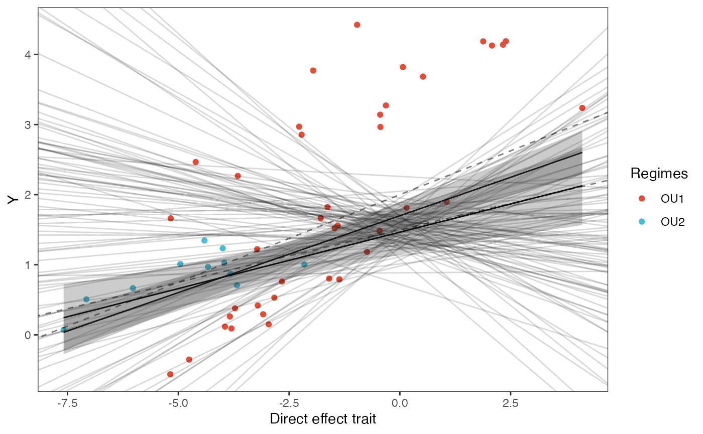

mu.link.Xa1<-function(x.seq){optima.post[,1]+x.seq*beta.post.Xa[,1]}
mu.link.Xa2<-function(x.seq){optima.post[,2]+x.seq*beta.post.Xa[,2]}

x.seq <- seq(from=min(dat$X_obs[,2]), to=max(dat$X_obs[,2]) , length.out=100)
mu.11 <- sapply(x.seq , mu.link.Xa1 )
mu.12 <- sapply(x.seq , mu.link.Xa2 )

mu.mean.11<-colMeans(mu.11)
mu.mean.12<-colMeans(mu.12)

mu.mean.11<-data.frame(as.numeric(mu.mean.11))
mu.mean.12<-data.frame(as.numeric(mu.mean.12))
names(mu.mean.11)<-"mu.mean.11"
names(mu.mean.12)<-"mu.mean.12"

mu.CI.11 <- apply( mu.11 , MARGIN=2, FUN=rethinking::PI , prob=0.89 )
mu.CI.12 <- apply( mu.12 , MARGIN=2, FUN=rethinking::PI , prob=0.89 )

mu.CI.11<-data.frame(t(data.frame(mu.CI.11)),x.seq)
mu.CI.12<-data.frame(t(data.frame(mu.CI.12)),x.seq)

names(mu.CI.11)<-c("min.5.5","max.94.5","x.seq")
names(mu.CI.12)<-c("min.5.5","max.94.5","x.seq")

df<-data.frame(Y=dat$Y_obs,X=dat$X_obs,Regimes=regimes_tip)
df11<-data.frame(x.seq,mu.mean.11)
df12<-data.frame(x.seq,mu.mean.12)

mypal <- ggsci::pal_npg("nrc", alpha = 0.7)(length(beta))
slope.plot.2<-ggplot2::ggplot()+  
  ggplot2::geom_point(data=df,ggplot2::aes(y=Y,x=X.Xa,color=Regimes))+
  ggplot2::geom_abline(intercept=optima.sims,slope=beta.sims,alpha=0.15)+ #Prior
  ggplot2::geom_abline(intercept=optima[1],slope=beta[1,2],alpha=0.5,linetype=2)+
  ggplot2::geom_abline(intercept=optima[2],slope=beta[2,2],alpha=0.5,linetype=2)+
  
  ggplot2::geom_line(data=df11,ggplot2::aes(x=x.seq,y=mu.mean.11),linetype=1)+
  ggplot2::geom_ribbon(data=mu.CI.11,ggplot2::aes(x=x.seq,ymin=min.5.5,ymax=max.94.5),linetype=2,alpha=0.25)+
  ggplot2::geom_line(data=df12,ggplot2::aes(x=x.seq,y=mu.mean.12),linetype=1)+
  ggplot2::geom_ribbon(data=mu.CI.12,ggplot2::aes(x=x.seq,ymin=min.5.5,ymax=max.94.5),linetype=2,alpha=0.25)+
  ggplot2::theme_bw()+
  ggplot2::theme(
    panel.grid.major = ggplot2::element_blank(),
    panel.grid.minor = ggplot2::element_blank())+
  
  #ggtitle("Prior vs. Posterior for Intercept and Slope")+
  ggplot2::ylab("Y") + ggplot2::xlab("Adaptive trait")+
  ggsci::scale_color_npg()

slope.plot.2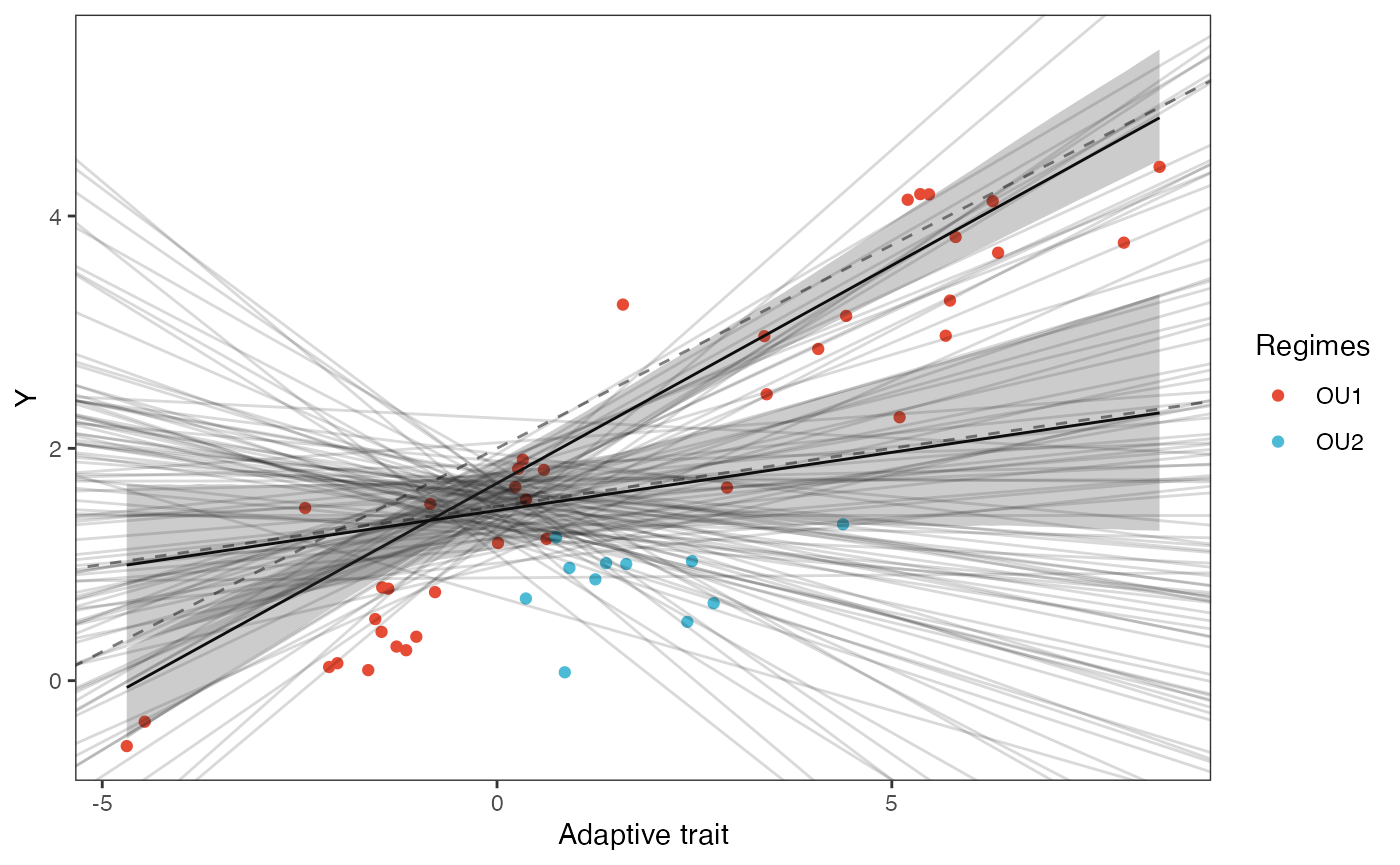

Now we run the Multilevel Multi-optima Direct Effect Adaptation Model with Varying Effects, look at the results, and rstan::extract the posterior

Next we will set the priors for the estimated parameters - for this model this includes the half-life, Vy, optima, and beta. For the latter two parameters we will use the results of the linear model to inform our priors.

############################################################################################################
#Set Priors
hl.prior<-c(log(0.25),0.75)
vy.prior<-20
optima.prior<-c(1.5,0.25) #Informed by linear model
beta.prior<-c(0,0.25) #Informed by linear model
sigma.prior<-c(0,1) #Informed by linear model

We will use the helper function blouch.reg.adapt.prep() to setup the dat file for Stan. Here “Z_adaptive” is the number of predictors, and “regimes” is the name of the regime column in trdata$dat.

############################################################################################################
dat<-blouch.reg.direct.adapt.mlm.prep(trdata,"Y_with_error","Y_error",c("Xd","Xa"),c("Xd_error","Xa_error"),Z_direct=1,Z_adaptive=1,"regimes",hl.prior,vy.prior,optima.prior,beta.prior,sigma.prior)

fit.reg.direct.adapt.mlm.ve<- rstan::sampling(object = blouch:::stanmodels$blouchOU_reg_direct_adapt_mlm_ve,data = dat,chains = 2,cores=2,iter=2000)
#> Found more than one class "stanfit" in cache; using the first, from namespace 'rstan'
#> Also defined by 'rethinking'
#> Found more than one class "stanfit" in cache; using the first, from namespace 'rstan'
#> Also defined by 'rethinking'
#> Warning: There were 374 divergent transitions after warmup. See
#> https://mc-stan.org/misc/warnings.html#divergent-transitions-after-warmup
#> to find out why this is a problem and how to eliminate them.
#> Warning: Examine the pairs() plot to diagnose sampling problems
#> Warning: Tail Effective Samples Size (ESS) is too low, indicating posterior variances and tail quantiles may be unreliable.
#> Running the chains for more iterations may help. See
#> https://mc-stan.org/misc/warnings.html#tail-ess

print(fit.reg.direct.adapt.mlm.ve,pars = c("hl","vy","optima","beta","sigma","Rho"))
#> Inference for Stan model: blouchOU_reg_direct_adapt_mlm_ve.
#> 2 chains, each with iter=2000; warmup=1000; thin=1; 
#> post-warmup draws per chain=1000, total post-warmup draws=2000.
#> 
#>           mean se_mean   sd  2.5%   25%  50%  75% 97.5% n_eff Rhat
#> hl        0.13    0.01 0.11  0.05  0.08 0.10 0.14  0.45   205 1.01
#> vy        0.01    0.00 0.01  0.00  0.00 0.01 0.02  0.05  1946 1.00
#> optima[1] 1.72    0.00 0.14  1.45  1.63 1.73 1.81  2.00  1068 1.00
#> optima[2] 1.54    0.01 0.27  0.94  1.38 1.56 1.71  2.02  1155 1.00
#> beta[1,1] 0.22    0.00 0.03  0.16  0.20 0.22 0.24  0.27  1855 1.00
#> beta[1,2] 0.38    0.01 0.07  0.32  0.35 0.37 0.39  0.59   194 1.01
#> beta[2,1] 0.18    0.00 0.05  0.07  0.15 0.19 0.22  0.27  1518 1.00
#> beta[2,2] 0.12    0.00 0.08 -0.04  0.07 0.12 0.17  0.27   958 1.00
#> sigma[1]  0.42    0.02 0.38  0.03  0.15 0.31 0.57  1.41   617 1.00
#> sigma[2]  0.25    0.01 0.29  0.02  0.06 0.15 0.34  1.04   795 1.00
#> sigma[3]  0.47    0.01 0.35  0.08  0.21 0.36 0.62  1.42  1532 1.00
#> Rho[1,1]  1.00     NaN 0.00  1.00  1.00 1.00 1.00  1.00   NaN  NaN
#> Rho[1,2]  0.01    0.01 0.31 -0.57 -0.21 0.01 0.24  0.60  1760 1.00
#> Rho[1,3]  0.02    0.01 0.32 -0.56 -0.21 0.02 0.24  0.62  2206 1.00
#> Rho[2,1]  0.01    0.01 0.31 -0.57 -0.21 0.01 0.24  0.60  1760 1.00
#> Rho[2,2]  1.00    0.00 0.00  1.00  1.00 1.00 1.00  1.00  1699 1.00
#> Rho[2,3]  0.02    0.01 0.31 -0.56 -0.20 0.02 0.24  0.63   854 1.00
#> Rho[3,1]  0.02    0.01 0.32 -0.56 -0.21 0.02 0.24  0.62  2206 1.00
#> Rho[3,2]  0.02    0.01 0.31 -0.56 -0.20 0.02 0.24  0.63   854 1.00
#> Rho[3,3]  1.00    0.00 0.00  1.00  1.00 1.00 1.00  1.00  1316 1.00
#> 
#> Samples were drawn using NUTS(diag_e) at Tue Oct  8 14:18:27 2024.
#> For each parameter, n_eff is a crude measure of effective sample size,
#> and Rhat is the potential scale reduction factor on split chains (at 
#> convergence, Rhat=1).
post<-rstan::extract(fit.reg.direct.adapt.mlm.ve)

Now we run the non-centered version of the Multilevel Multi-optima Direct Effect Adaptive Model with Varying Effects

fit.reg.direct.adapt.mlm.ve.nc<- rstan::sampling(object = blouch:::stanmodels$blouchOU_reg_direct_adapt_mlm_ve_nc,data = dat,chains = 2,cores=2,iter=2000)
#> Found more than one class "stanfit" in cache; using the first, from namespace 'rstan'
#> Also defined by 'rethinking'
#> Found more than one class "stanfit" in cache; using the first, from namespace 'rstan'
#> Also defined by 'rethinking'
#> Warning: There were 111 divergent transitions after warmup. See
#> https://mc-stan.org/misc/warnings.html#divergent-transitions-after-warmup
#> to find out why this is a problem and how to eliminate them.
#> Warning: Examine the pairs() plot to diagnose sampling problems

print(fit.reg.direct.adapt.mlm.ve.nc,pars = c("hl","vy","optima","beta","sigma","L_Rho"))
#> Inference for Stan model: blouchOU_reg_direct_adapt_mlm_ve_nc.
#> 2 chains, each with iter=2000; warmup=1000; thin=1; 
#> post-warmup draws per chain=1000, total post-warmup draws=2000.
#> 
#>            mean se_mean   sd  2.5%   25%  50%  75% 97.5% n_eff Rhat
#> hl         0.13    0.00 0.12  0.05  0.07 0.10 0.15  0.43   833 1.00
#> vy         0.01    0.00 0.01  0.00  0.00 0.01 0.02  0.05  2368 1.00
#> optima[1]  1.71    0.00 0.14  1.42  1.63 1.72 1.80  1.98  1572 1.00
#> optima[2]  1.57    0.01 0.25  1.05  1.43 1.59 1.73  2.04  1666 1.00
#> beta[1,1]  0.22    0.00 0.03  0.17  0.20 0.22 0.24  0.27  1434 1.00
#> beta[1,2]  0.38    0.00 0.08  0.32  0.35 0.37 0.39  0.57   752 1.00
#> beta[2,1]  0.19    0.00 0.05  0.08  0.16 0.19 0.22  0.28  1471 1.00
#> beta[2,2]  0.12    0.00 0.08 -0.03  0.07 0.12 0.17  0.27  1334 1.00
#> sigma[1]   0.39    0.01 0.37  0.02  0.12 0.28 0.56  1.40   862 1.00
#> sigma[2]   0.18    0.01 0.24  0.00  0.04 0.10 0.22  0.87   658 1.01
#> sigma[3]   0.37    0.01 0.27  0.07  0.17 0.28 0.47  1.10   457 1.00
#> L_Rho[1,1] 1.00     NaN 0.00  1.00  1.00 1.00 1.00  1.00   NaN  NaN
#> L_Rho[1,2] 0.00     NaN 0.00  0.00  0.00 0.00 0.00  0.00   NaN  NaN
#> L_Rho[1,3] 0.00     NaN 0.00  0.00  0.00 0.00 0.00  0.00   NaN  NaN
#> L_Rho[2,1] 0.03    0.01 0.43 -0.77 -0.32 0.02 0.36  0.79  1947 1.00
#> L_Rho[2,2] 0.89    0.00 0.13  0.54  0.85 0.94 0.98  1.00   788 1.00
#> L_Rho[2,3] 0.00     NaN 0.00  0.00  0.00 0.00 0.00  0.00   NaN  NaN
#> L_Rho[3,1] 0.07    0.01 0.40 -0.71 -0.23 0.08 0.39  0.79  1599 1.00
#> L_Rho[3,2] 0.07    0.01 0.42 -0.75 -0.25 0.09 0.42  0.82  1423 1.00
#> L_Rho[3,3] 0.79    0.01 0.17  0.37  0.69 0.83 0.92  0.99   815 1.00
#> 
#> Samples were drawn using NUTS(diag_e) at Tue Oct  8 14:21:01 2024.
#> For each parameter, n_eff is a crude measure of effective sample size,
#> and Rhat is the potential scale reduction factor on split chains (at 
#> convergence, Rhat=1).
post<-rstan::extract(fit.reg.direct.adapt.mlm.ve.nc)

From there the posteriors should be explored, compared to the priors, etc. following the methods above.